 EA4FSI
| Type | Resistively loaded Sloping Vee dipole |
|---|---|
| Design | N/A |
| Impedance | 235 Ω |
| Simulation | MMANA-GAL |
| Band | Broadband HF |

1. Antenna design and modelling.
In this Sloping Vee design, each arm is 12 m long and terminates in a 470 Ω resistive load connected to ground (Fig. 1). The mast must be at least 6 m high. A ladder-line transmission line with a suitable characteristic impedance should be used, together with a 4:1 balun. An antenna tuner is recommended, particularly for automatic link establishment (ALE) operation.
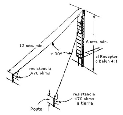
Figure 2 shows the antenna modelled in MMANA-GAL.
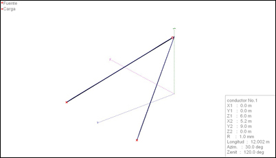
The feed point is located on the Z-axis, 6 m above ground. The two dipole arms extend from this point, forming a 30° angle bisected by the Y-axis. A 470 Ω resistive load is connected at the far end of each arm.
2. Simulation results.
This section presents the MMANA-GAL simulation results, including calculated standing-wave ratios (SWR) and radiation patterns at the frequencies studied.
2.1. Standing-wave ratio (SWR).
Figure 3 shows the calculated SWR referenced to 200 Ω, corresponding to a 50 Ω transmitter connected through a 4:1 impedance-transforming balun.
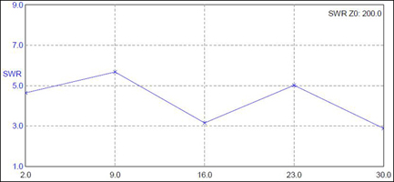
Although the SWR is relatively low, the simulation indicates that an antenna tuner is still required.
2.2. Radiation patterns.
Figure 4 shows the simulated radiation patterns at frequencies from 2 to 10 MHz.
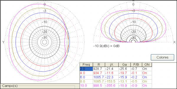
Figure 5 shows the simulated radiation patterns at frequencies from 11 to 20 MHz.
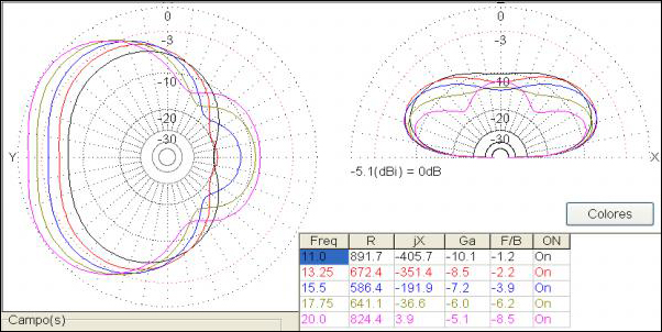
The antenna is directional, although its front-to-back ratio is relatively low. Maximum radiation occurs approximately along the bisector of the angle formed by the two arms. Losses occur throughout the operating band and become more pronounced at lower frequencies. Although the antenna has relatively low efficiency, it offers the advantage of a low SWR across the HF band.
The antenna is not recommended for near-vertical incidence skywave (NVIS) operation because of its low gain at lower frequencies.