


Welcome |

Main → HF Radio Resource Center → HF & Space Weather Panel
Welcome to the HF Radio and Space Weather Dashboard, a resource for the analysis of the interaction Sun-Earth and the propagation status in the HF band, with applications to radio communications.
This is an educational, non-commercial website. All displayed data is property of their authors and credit and hyperlinks to the corresponding sources are provided. If you want to contact the webmaster, please use this form.
Please choose an option:
 TOC |
 Español |
 Français |
 Mobile Version |
 Manual (ESP) |
 HF Central |
Current Space Weather 
 |
 |
 |
< < ALERTS | |
| Radio Blackout | Geomagnetic Storm | Solar Radiation Storm | ||
| < < 24-H FCST | ||||
| < < 48-H FCST | ||||
| < < 72-H FCST | ||||
| Radio Blackout R1-R3 Probability |
Radio Blackout R4-R5 Probability |
Geomagnetic Storm Probability |
Solar Radiation Storm Probability S1> | |
Updated every 5 minutes. Source: NOAA/SWPC |
||||
 |
 |
 |
 |
|
| HF Comms Warning | Current HF Fadeout | HF Fadeout Warning | Polar Absorption (PCA) | |
Source: Australian Space Weather Alert System |
||||
Source: NOAA/SWPC - DRAP2

Source: NOAA/SWPC
| Solar Wind | |||
 |
 |
 |
 |
| Interplanetary Magnetic Field (IMF) and Solar Ionosphere Potential | |||
 |
 |
 |
 |
Source: Rice University
Table of Contents
 Solar |
 Sun-Earth |
 Solar |
 Geomagnetic |
 Ionosphere Status |
 Radio Communications |
 Aurorae |
 Links |
 HF Glossary (ES) |
User's Manual (ES) |
HF Central |
 Technical Articles |
 EA4FSI Home |
 Contact Form |
The space weather affects a variety of services on Earth, such as radio communications, radionavigation systems or even the commercial airline routes. This web site proposes a visit arranged in a sequential way, starting with the analysis of the activity in the Sun itself. Then our journey will go on through the Solar System, following the solar radiation, the solar wind and the interplanetary magnetic field, until they reach the Earth's magnetosphere. Finally, we will see their effects when they reach the Earth at the end of this trip, in the form of solar radiation storms and geomagnetic storms, as well as their associated phenomena such as ionospheric perturbations and aurorae, putting an special emphasis on the impact on radio communications.
All along our trip, we will analyze real-time data provided by several Agencies and Universities that monitor the space weather, using both spacecrafts and terrestrial observatories, such as NOAA, NASA, JPL, ESA, Australian BOM, DLR and SIDC, among others.

Solar Activity
Solar X-Rays | Reports | Pictures of the Sun | Solar Flux Index and Sunspots
The Sun is our Solar System's star, a yellow dwarf star, with an approximate age of 4,6 billion years and a radius of around 696.340 km. The Sun is composed mainly of hydrogen (90%) and helium (10%), but several other elements such as carbon, oxygen and iron are present as well.
In the Sun's inner region, the temperature and the density are so high that hydrogen atoms suffer nuclear fusion. This process releases a huge amount of energy and produces helium. The energy is propagated towards the surface in the form of X-rays and other radiation types, generating electric currents which have associated strong magnetic fields.
The dynamic nature of these processes causes a variety of phenomena, such as flares, prominences, coronal holes or coronal mass ejections, where the radiation, the magnetic fields and solar particles are projected towards the space. Depending on how and where these phenomena are generated, they might reach the Earth and the spacecrafts orbiting around it.
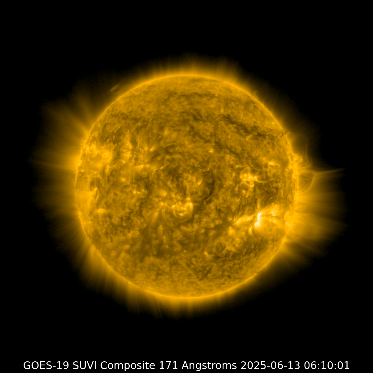
Source: NOAA/SWPC - GOES 16 SUVI
Actividad Solar
Solar X-Ray Flux & Solar Flares
The radiation resulting from the nuclear fusion processes within the Sun travels throughout the space and ultimately reaches the Earth. Part of this radiation contains enough energy so as to excite the oxygen and hydrogen molecules in the ionosphere, a layer of the atmosphere located at an altitude between 50-965 km (30-600 mi), inducing them to oscillate. This oscillation may cause those molecules to be dissociated into two atoms, even detaching some of their electrons, in a process called ionization. The most ionizing radiations generated by the Sun are within the range of the UV-rays (wavelength between 20-300 angstroms) and the X-Rays (wavelength between 8-20 angstroms). As a result of ionization, the electron density in the ionosphere increases, causing the absorption of radio waves in the HF band. This natural phenomena may hinder the setup of radio communications, even causing total radio blackouts. The following graphs show near real-time data of the ionizing radiation density flux in the X-Ray band, coming from the Sun and measured by the NOAA GOES-16 and GOES-17 spacecrafts.
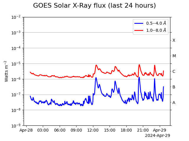
Source: NOAA/SWPC - GOES-16 and GOES-17 spacecrafts
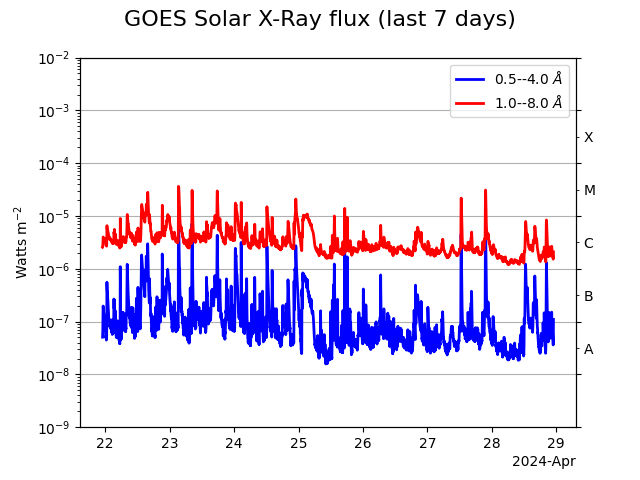
Source: NOAA/SWPC - GOES-16 and GOES-17 spacecrafts

The plots show real-time data of the ionizing radiation density flux (watts per square meter) in the X-Ray band, coming from the Sun and directed towards the Earth, as measured by the GOES-16 and GOES-17 spacecrafts. The peaks correspond to solar flares, that unleash huge amounts of X-Ray radiation. The rightmost scale shows the intensity of solar flares as a function of the measured radiation flux density: threshold A and B indicate normal flares. The C threshold is an indicator of a small solar flare, M is related to medium flares, X with big flares and beyond X indicates a so far unseen flare. The higher values are usually registered during periods of high solar activity within the 11-year solar cicle. The higher the intensity of the solar X-Ray emission, the greater the radio waves attenuation due to absorption in the HF band, caused by ionization within the ionosphere. In case of a major solar flare, please check the Spectrum Monitors and the HF Absorption Levels, which may be significant during intervals of minutes to hours. The plots have been generated with raw data provided by NOAA, using the SunPy Python package, a comprehensive data analysis environment for solar physics.
![]() ASWAS: Recent flare and fadeout information (larger than C8 only).
ASWAS: Recent flare and fadeout information (larger than C8 only).
Solar Activity
Solar Activity Reports
Source: Solar Activity Plot - Australian Space Weather Alert System
![]() Big Bear Solar Observatory: Daily solar activity reports.
Big Bear Solar Observatory: Daily solar activity reports.
![]() Big Bear Solar Observatory: Solar activity warnings.
Big Bear Solar Observatory: Solar activity warnings.
Solar Activity
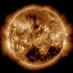
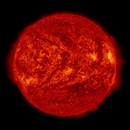
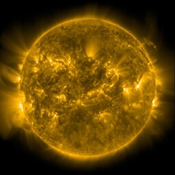
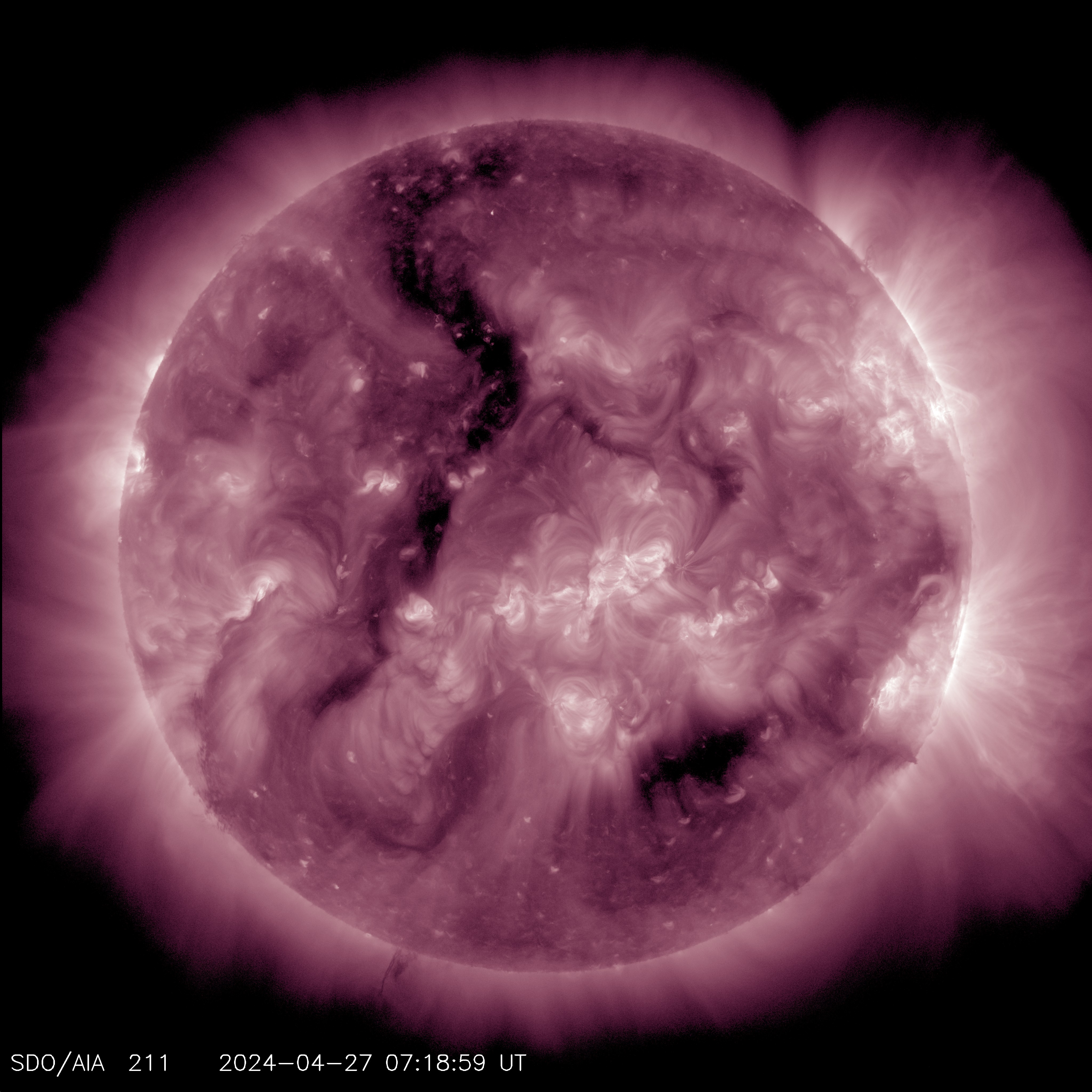
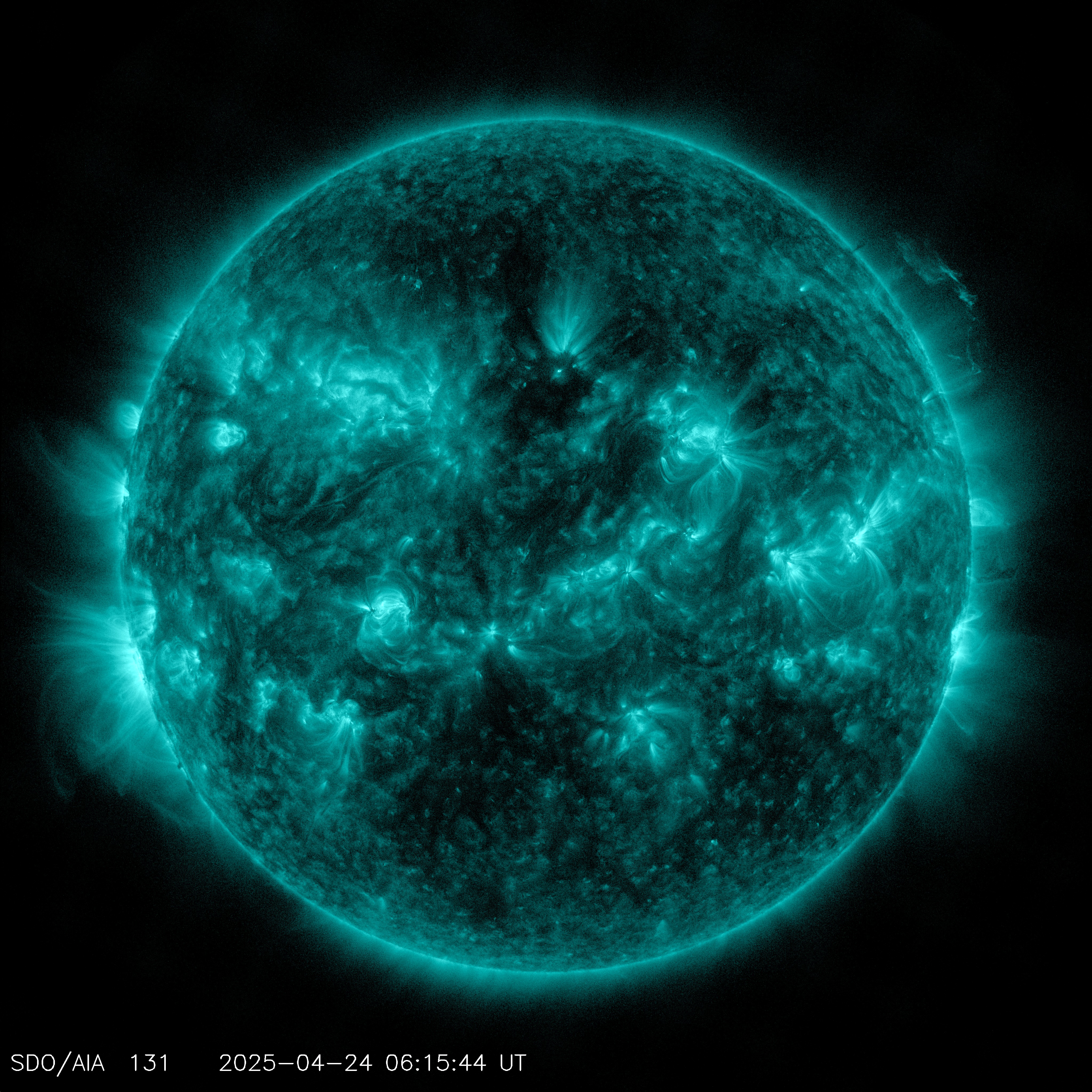
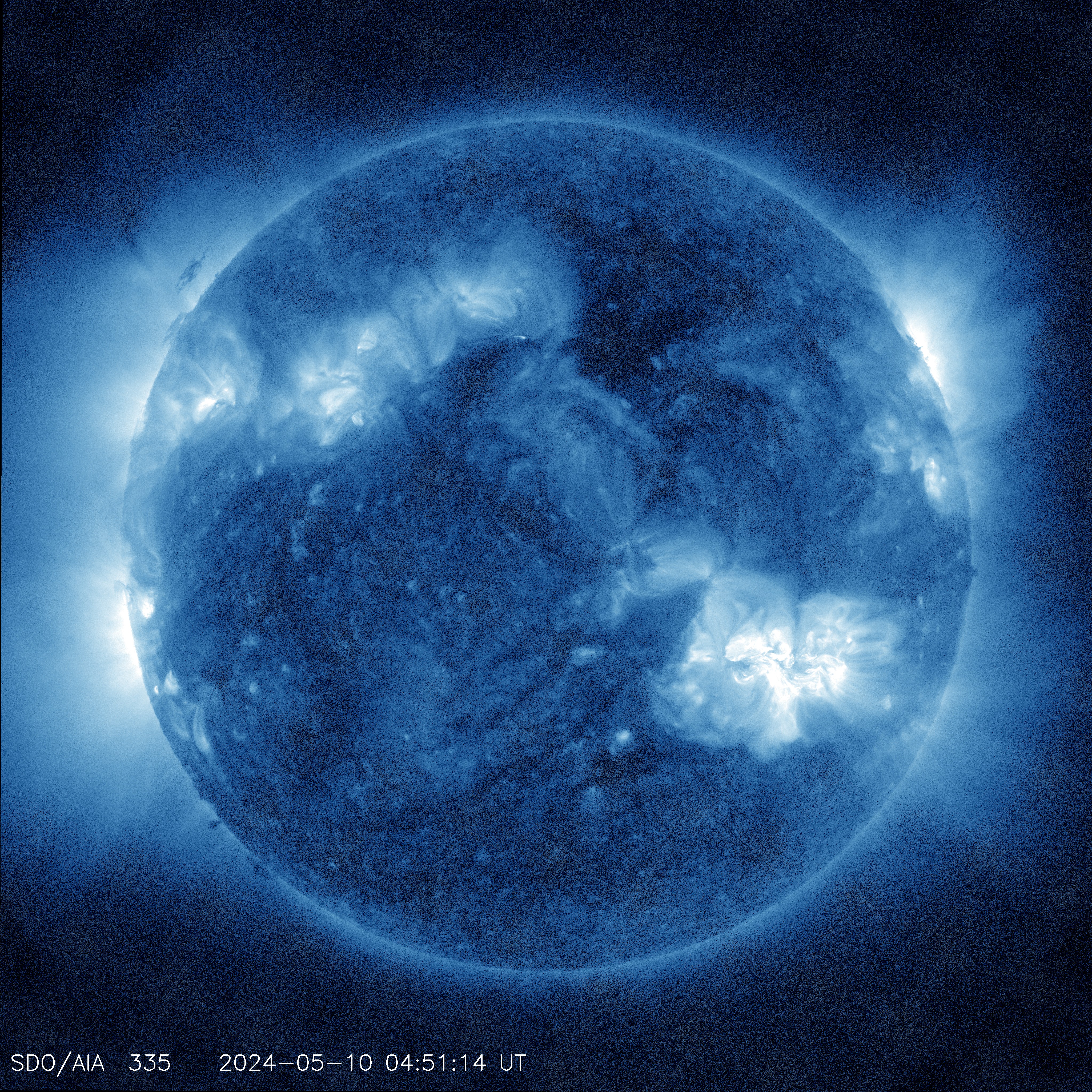
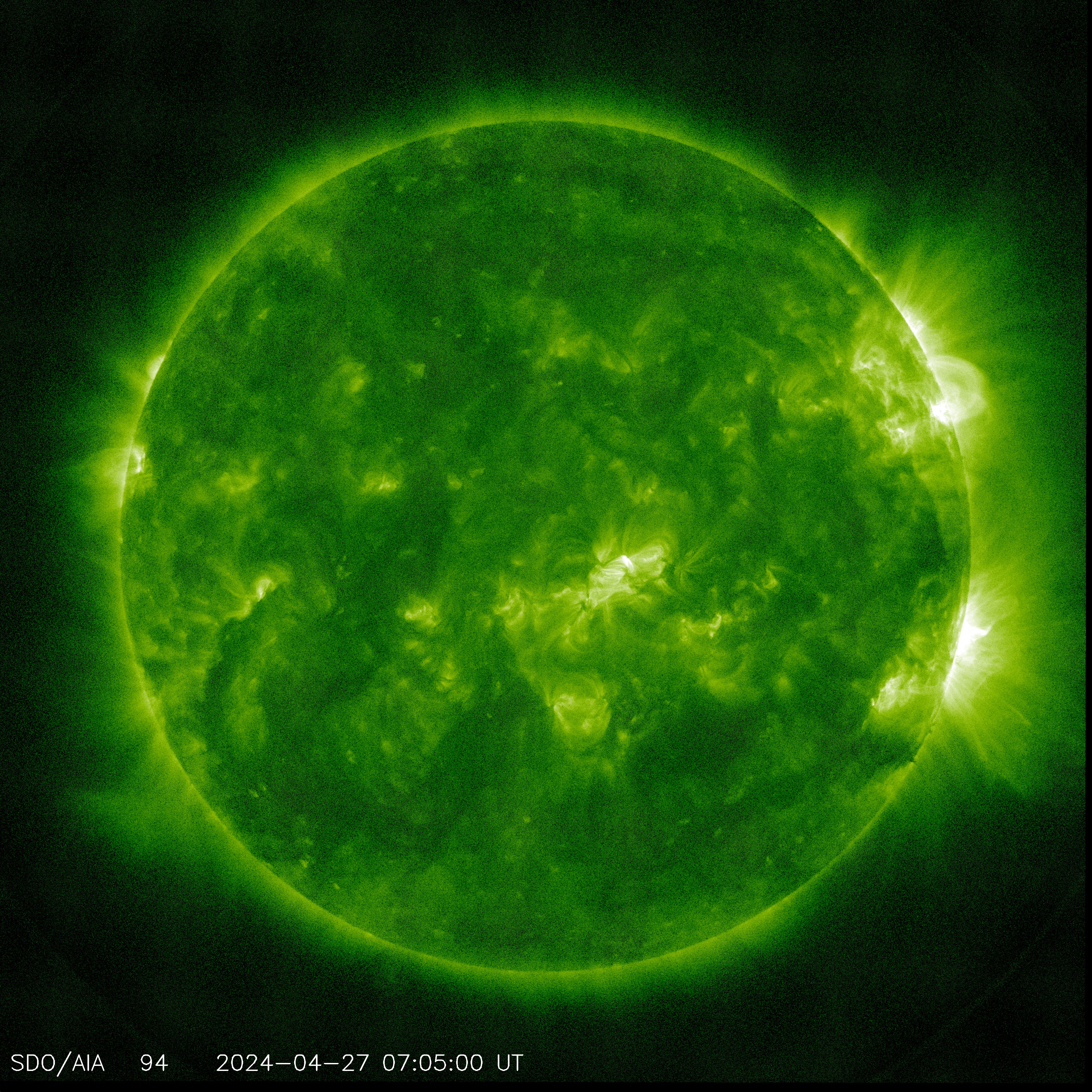
Pictures of the Sun

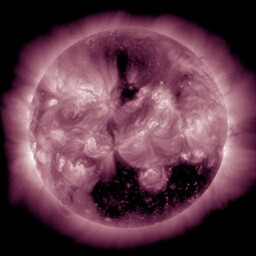
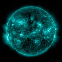
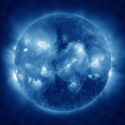
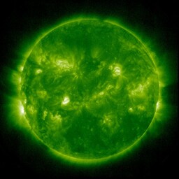
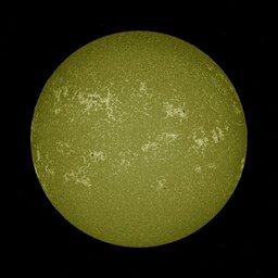
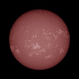
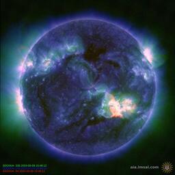
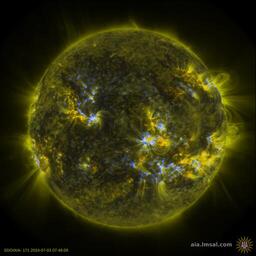
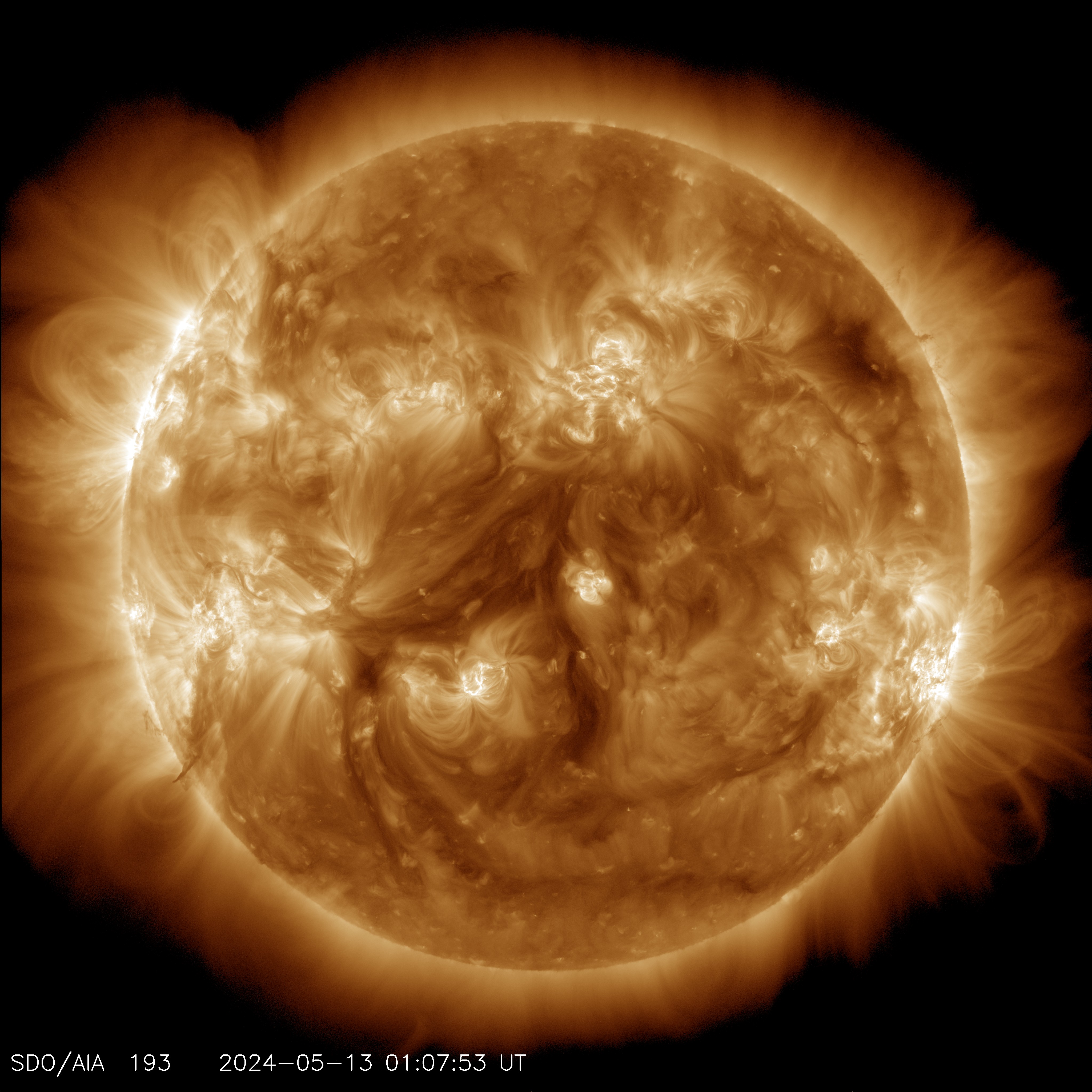
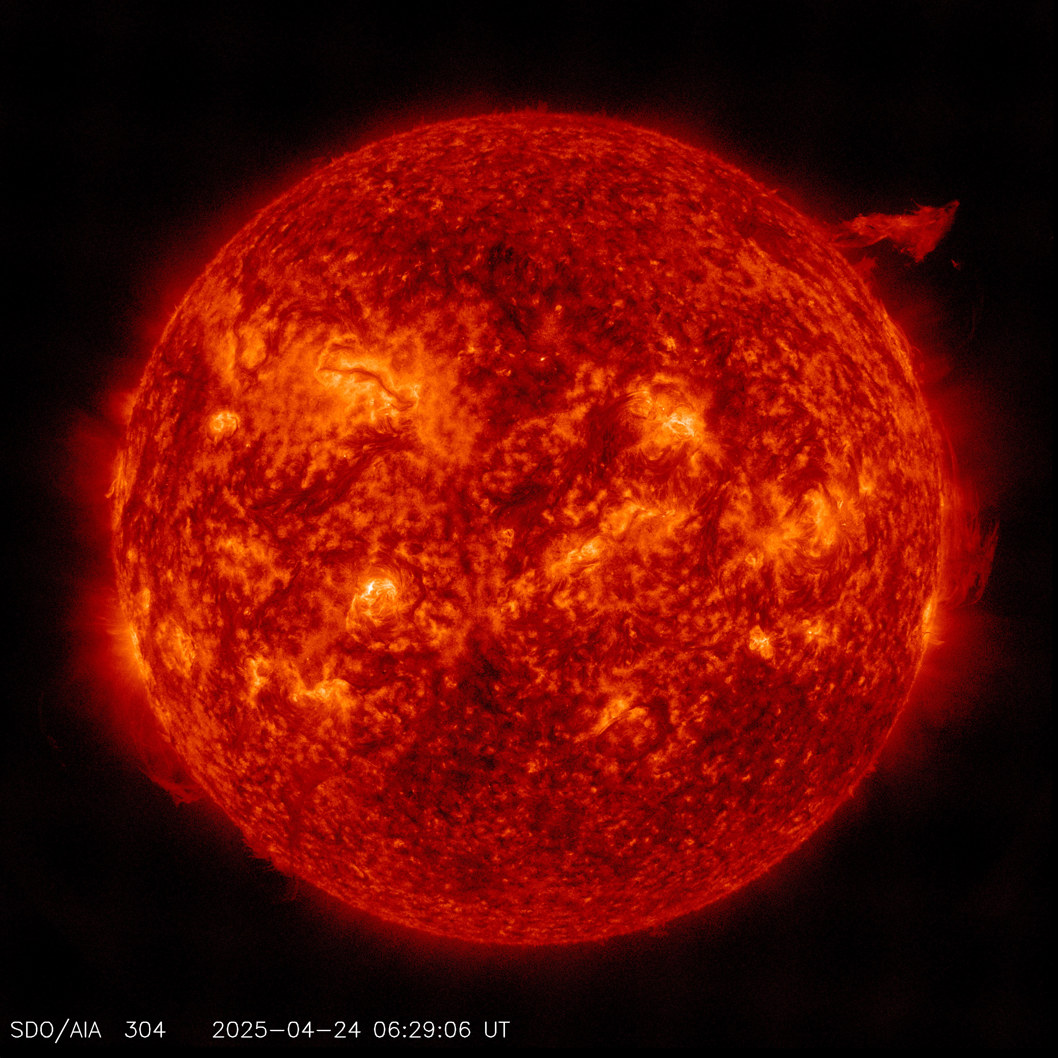
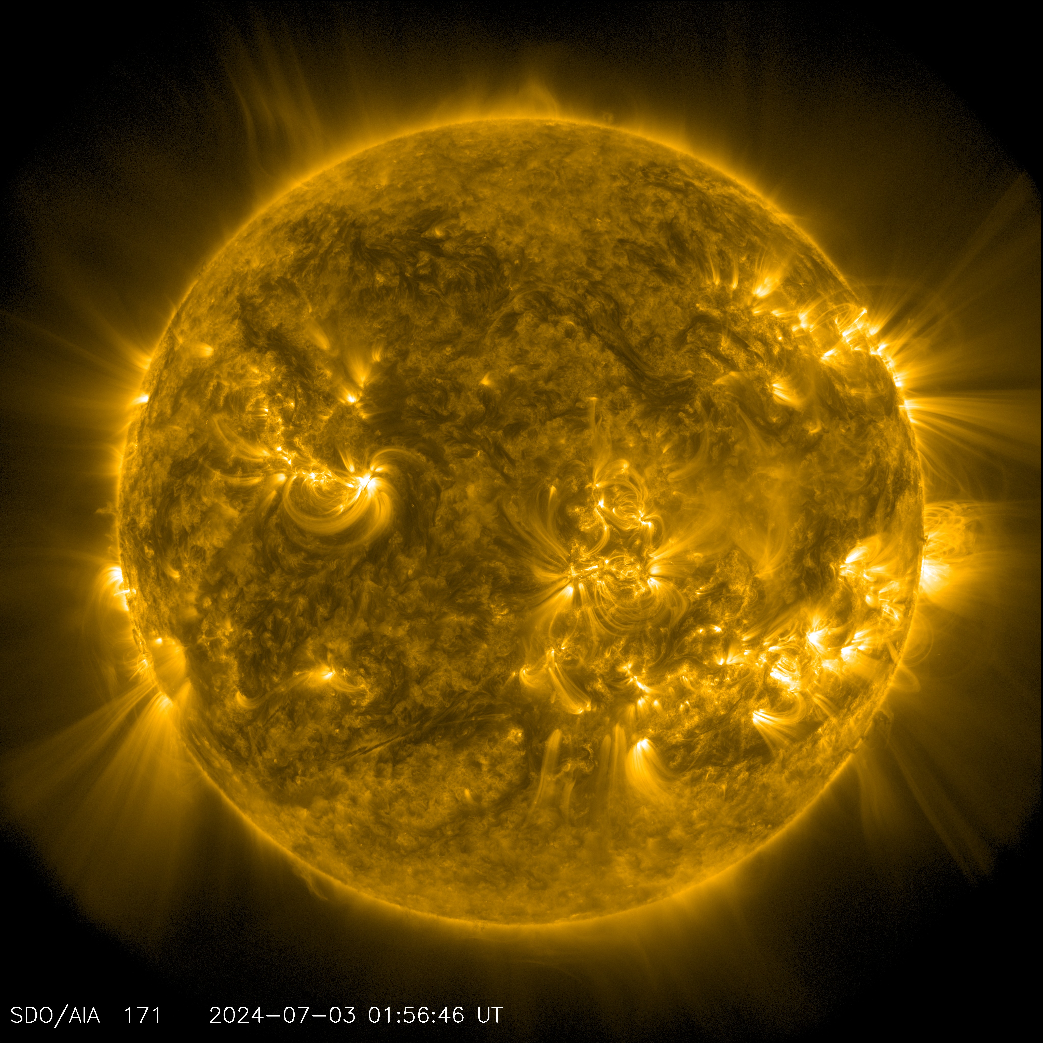
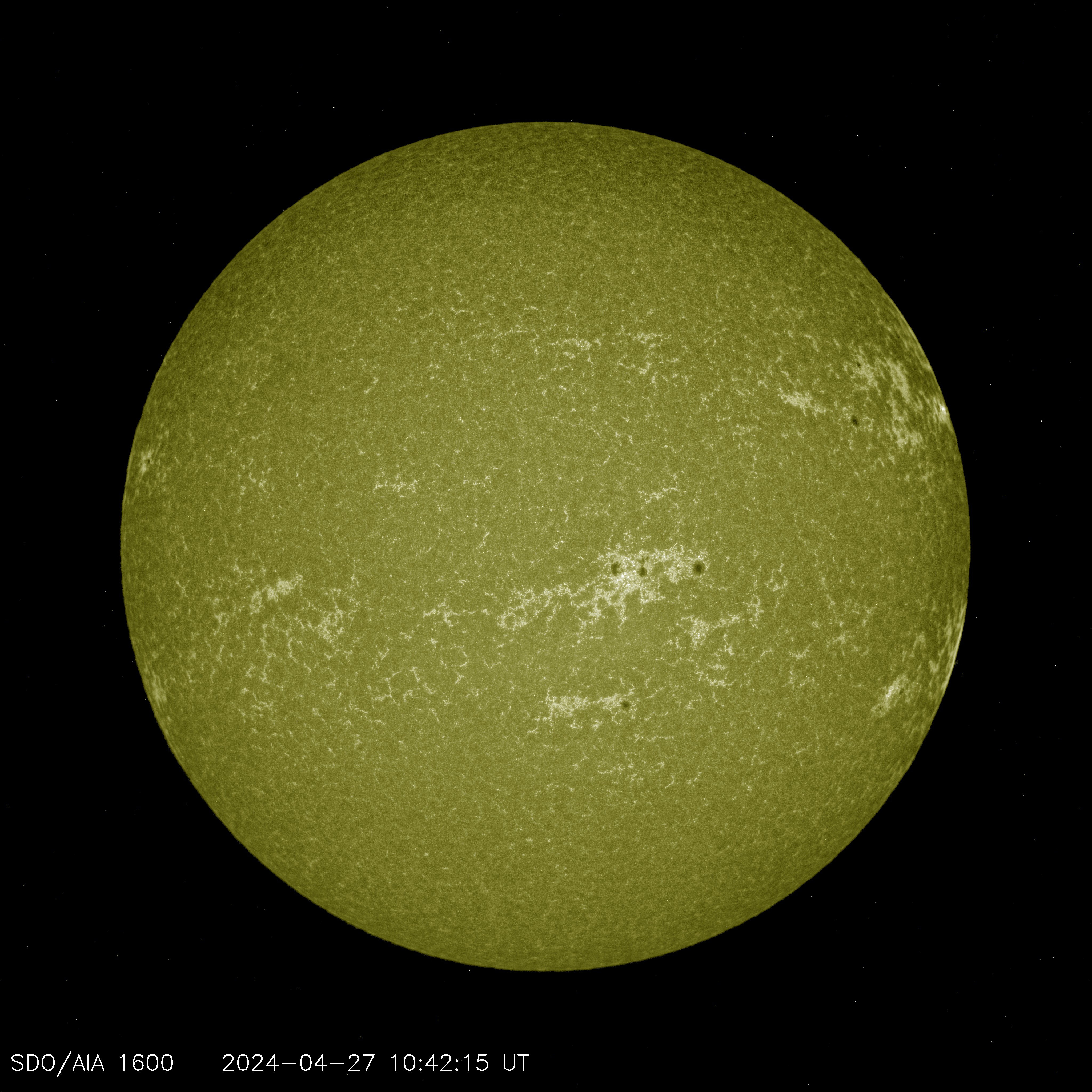
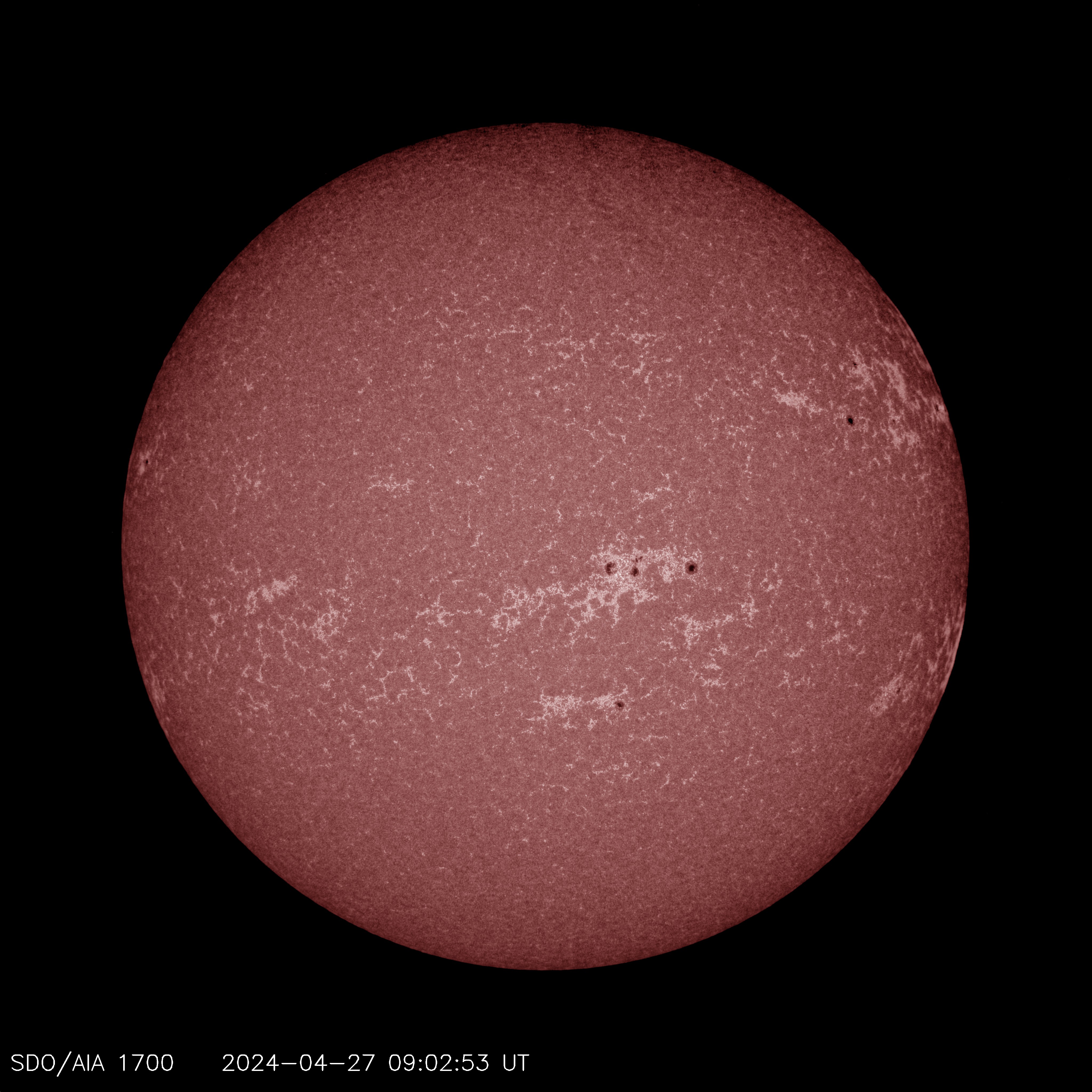
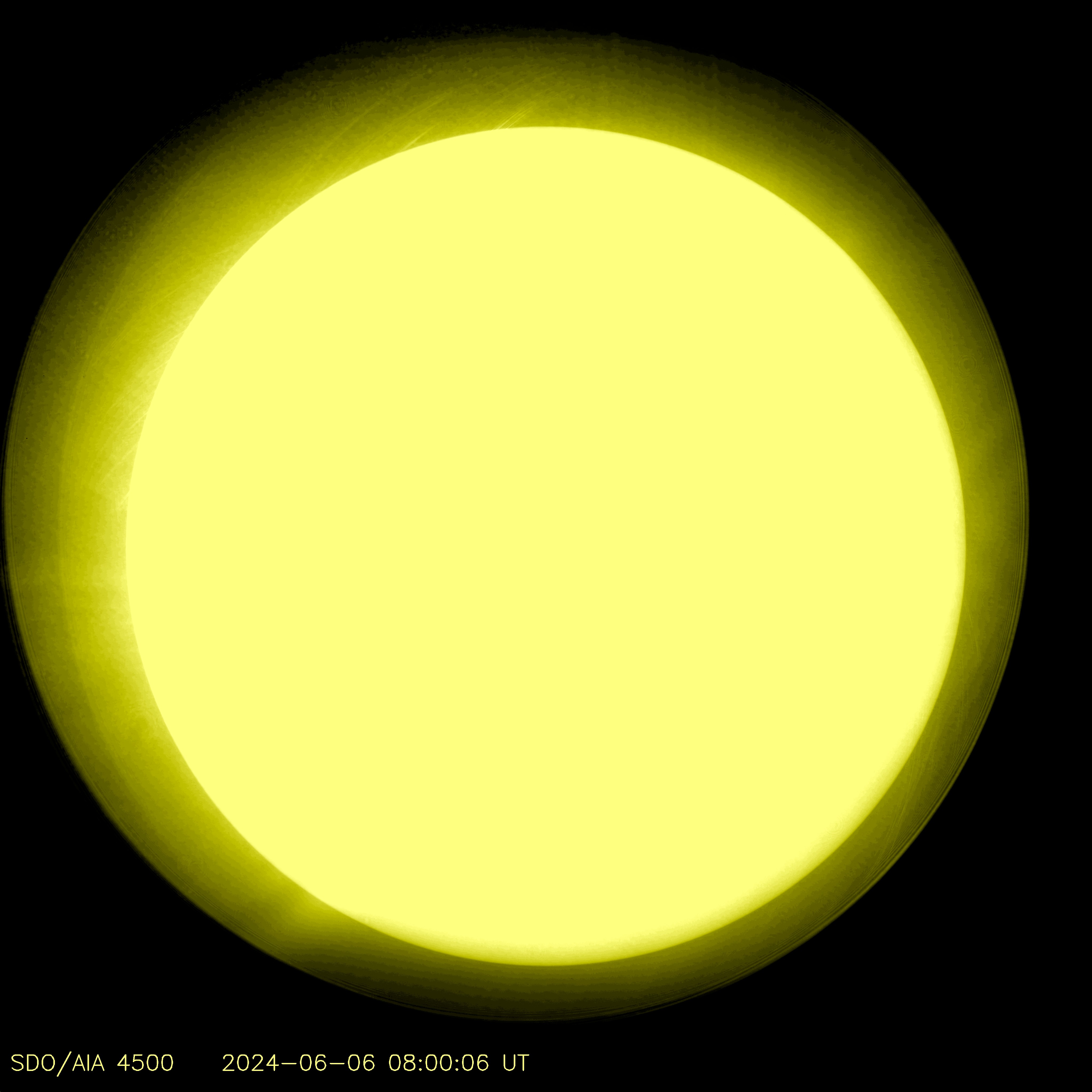
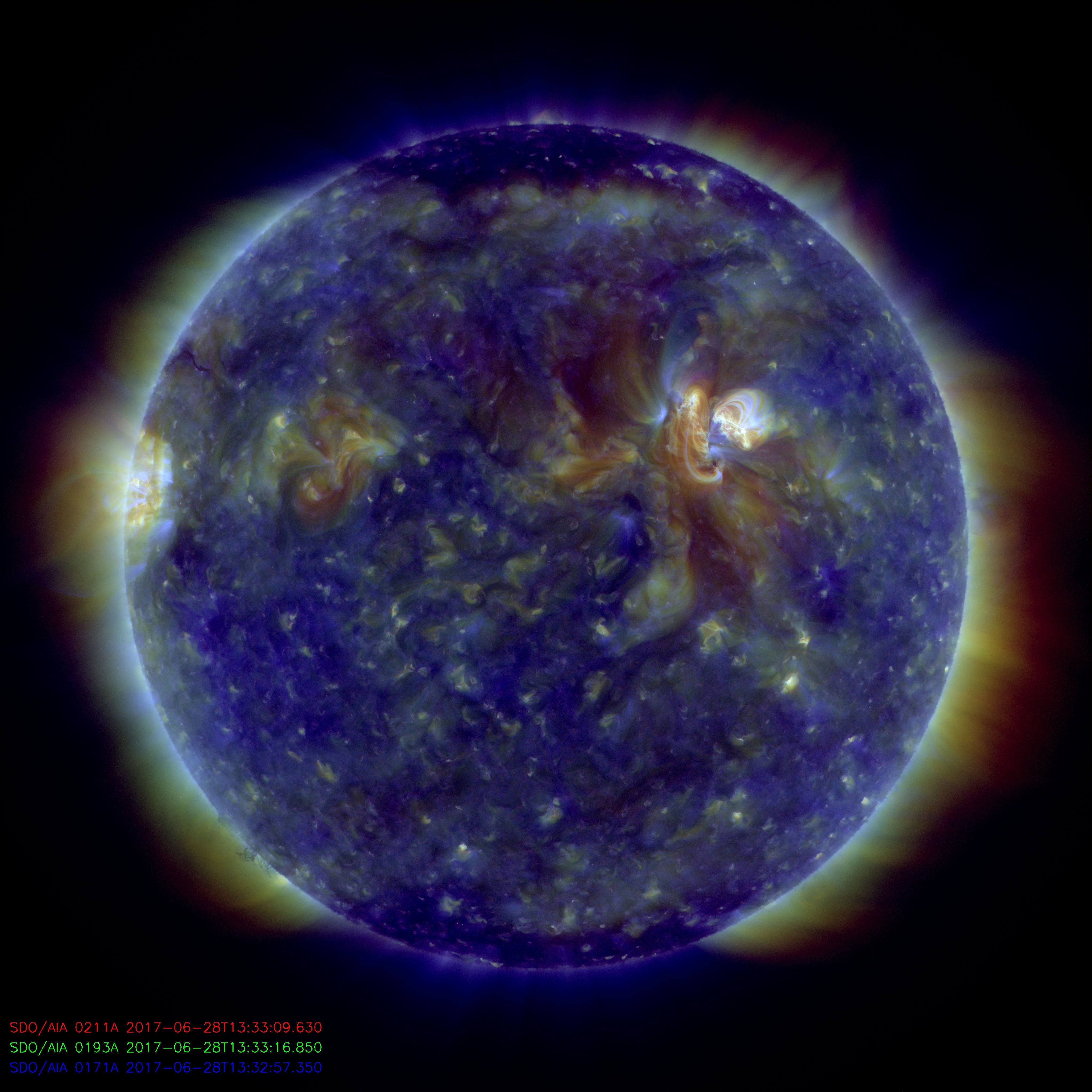
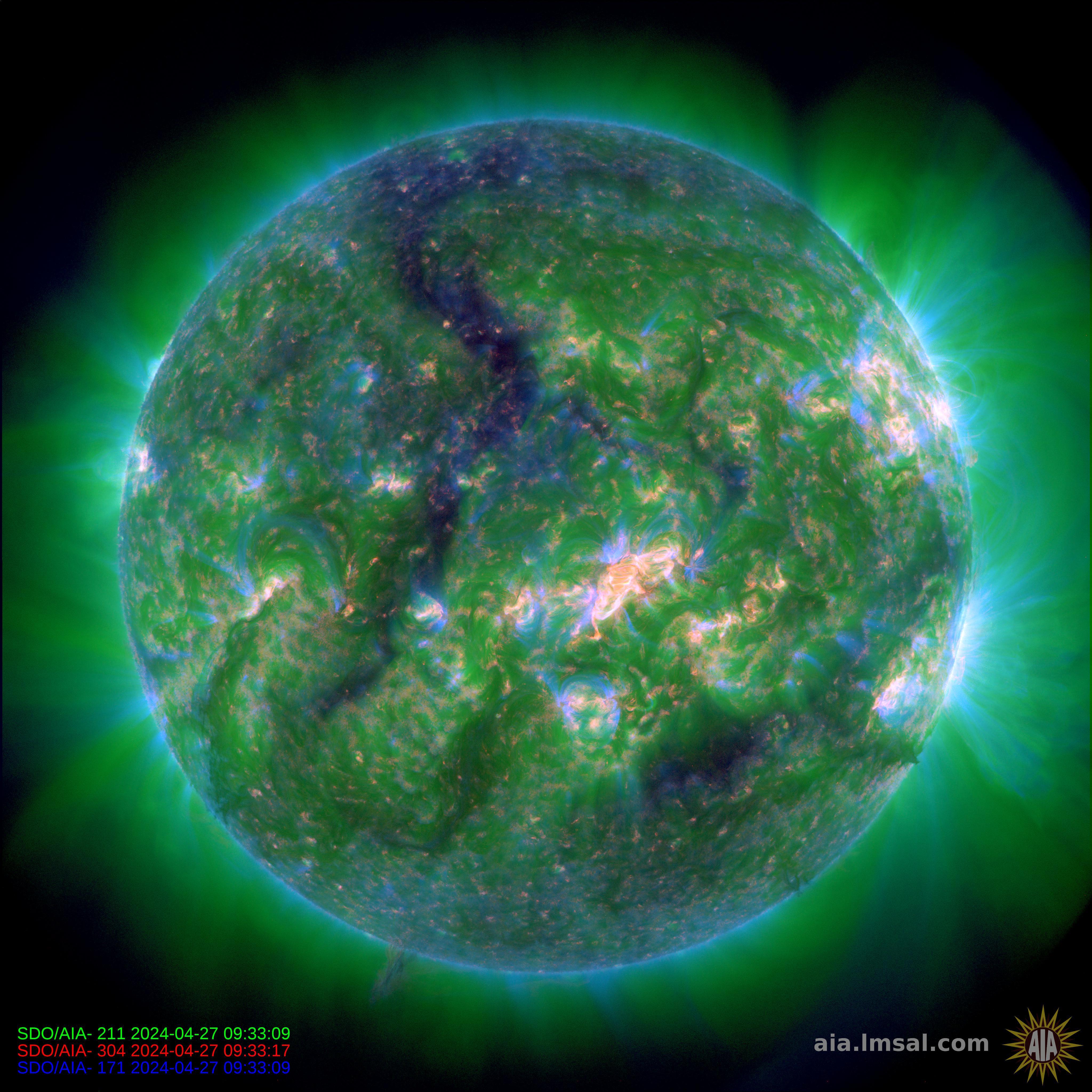
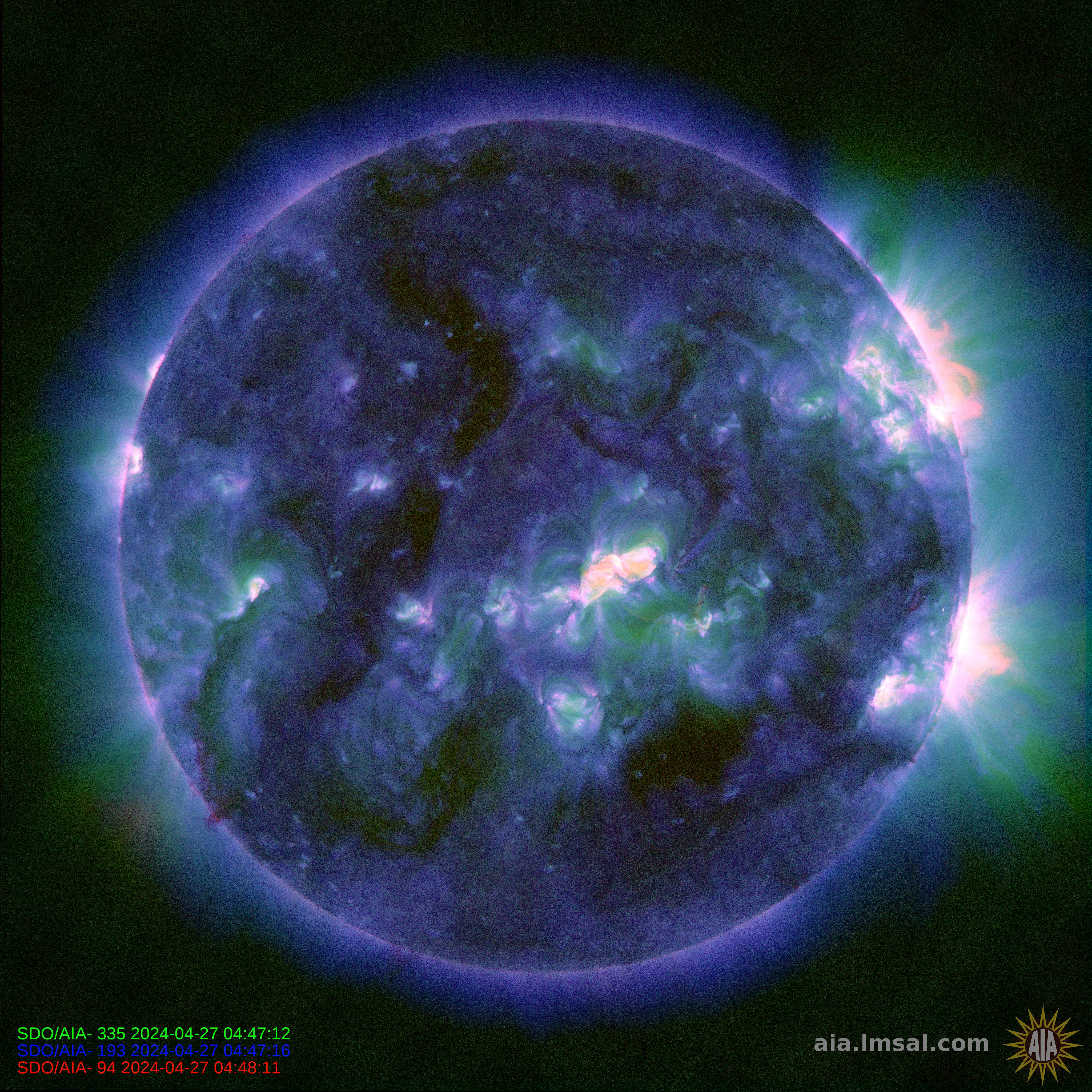
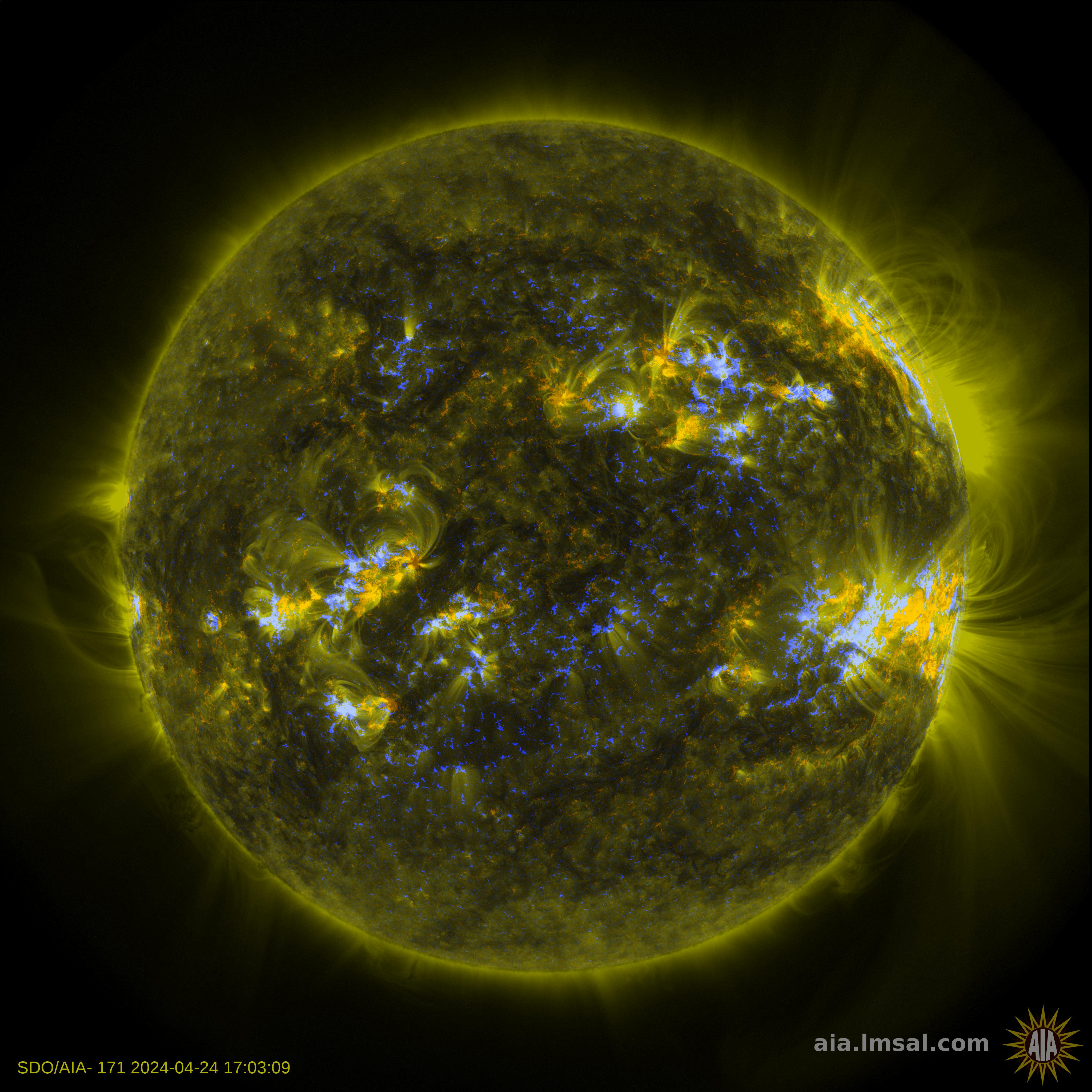
Current solar images taken every 10 seconds by the Atmospheric Image Assembly (AIS) instrument of the NASA's Solar Dynamics Observatory (SDO), at different wavelengths. For each picture, a high resolution version and a movie showing the last 48 hours pictures are available. Courtesy of NASA/SDO and the AIA, EVE, and HMI science teams.
 High resolution | Video |
 High resolution | Video |
 High resolution | Video |
 High resolution | Video |
 High resolution | Video |
 High resolution | Video |
 High resolution | Video |
 High resolution | Video |
 High resolution | Video |
 High resolution | Video |
|
|
|
|


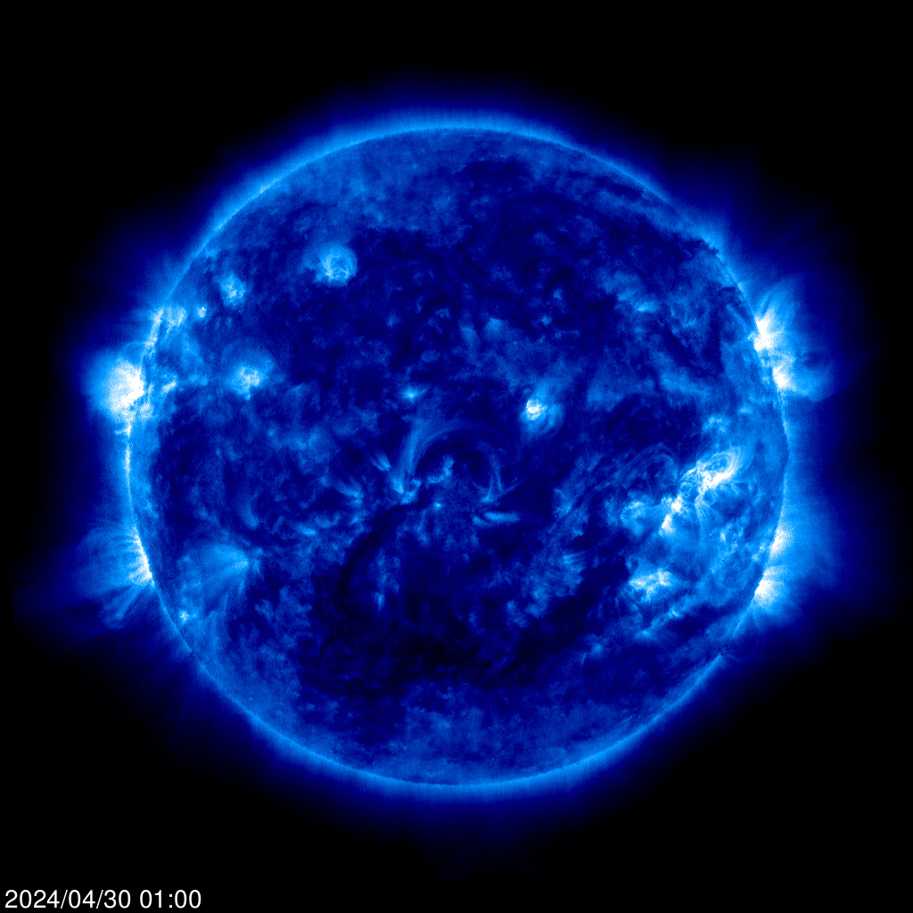
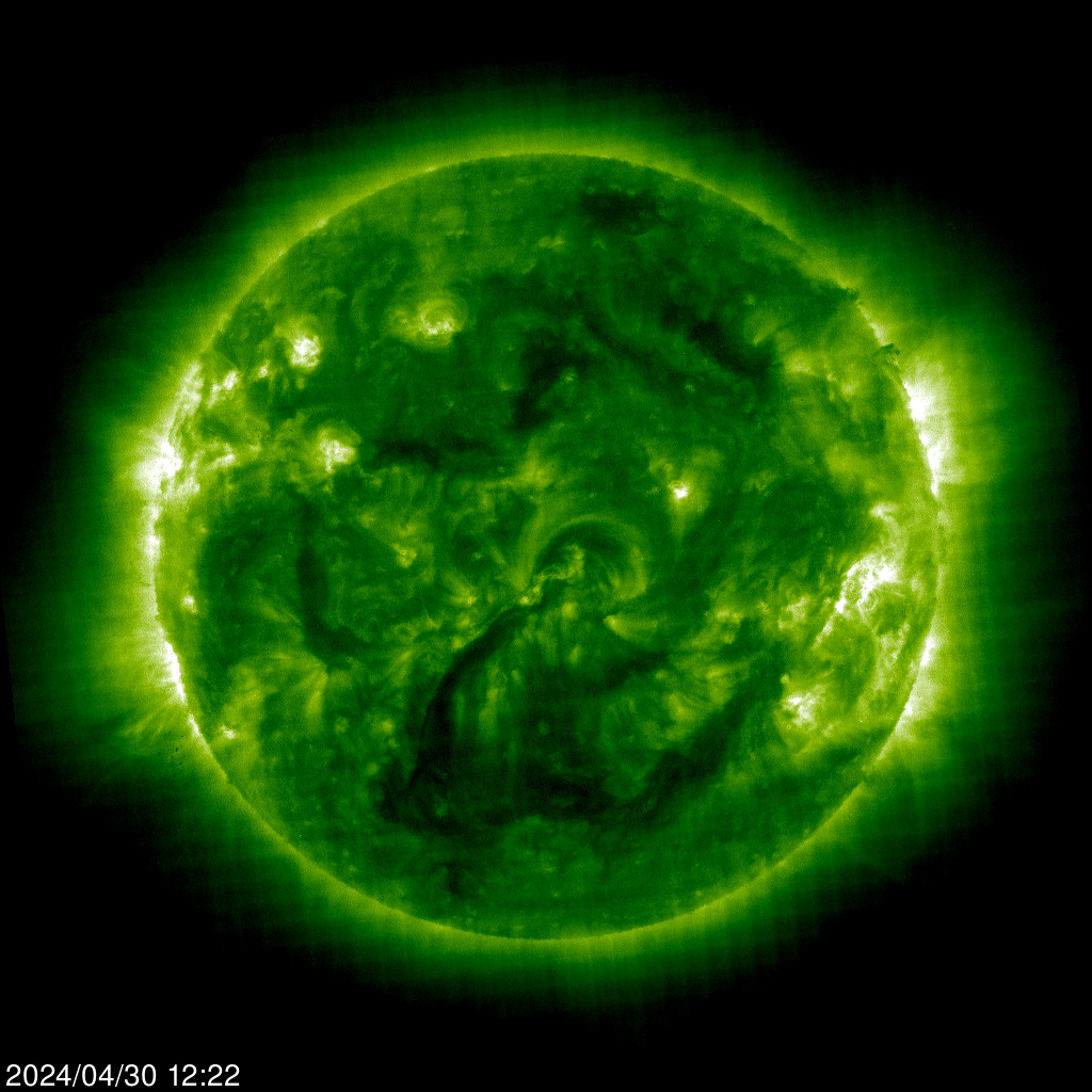
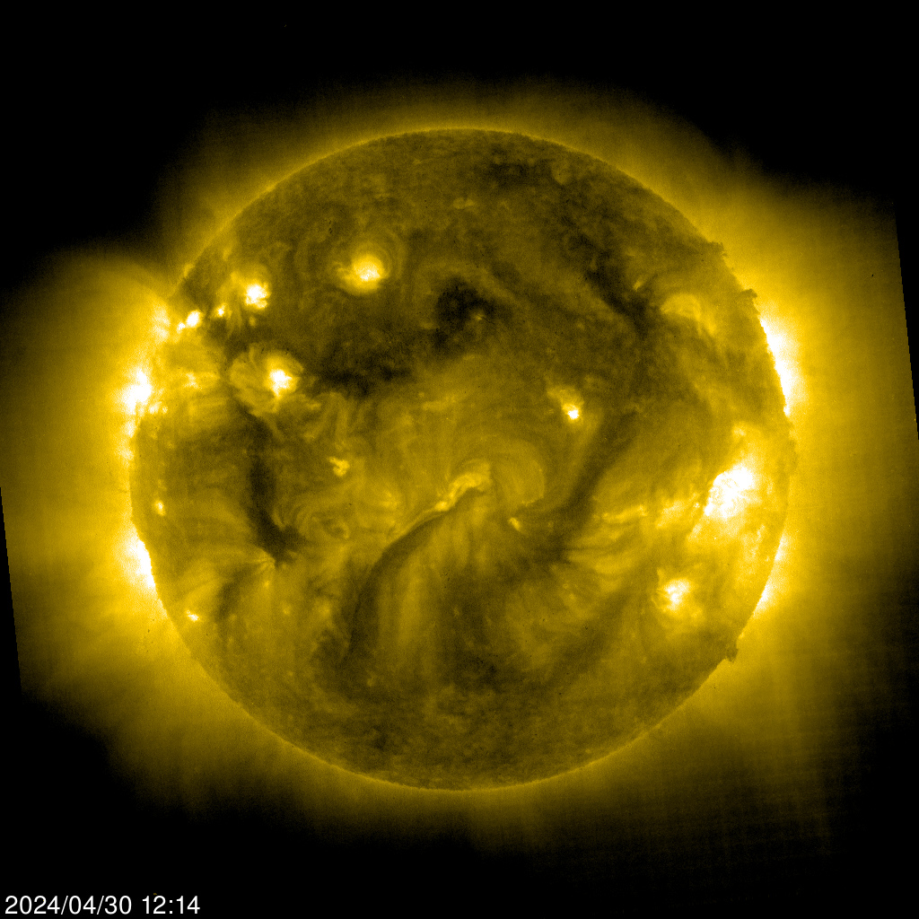
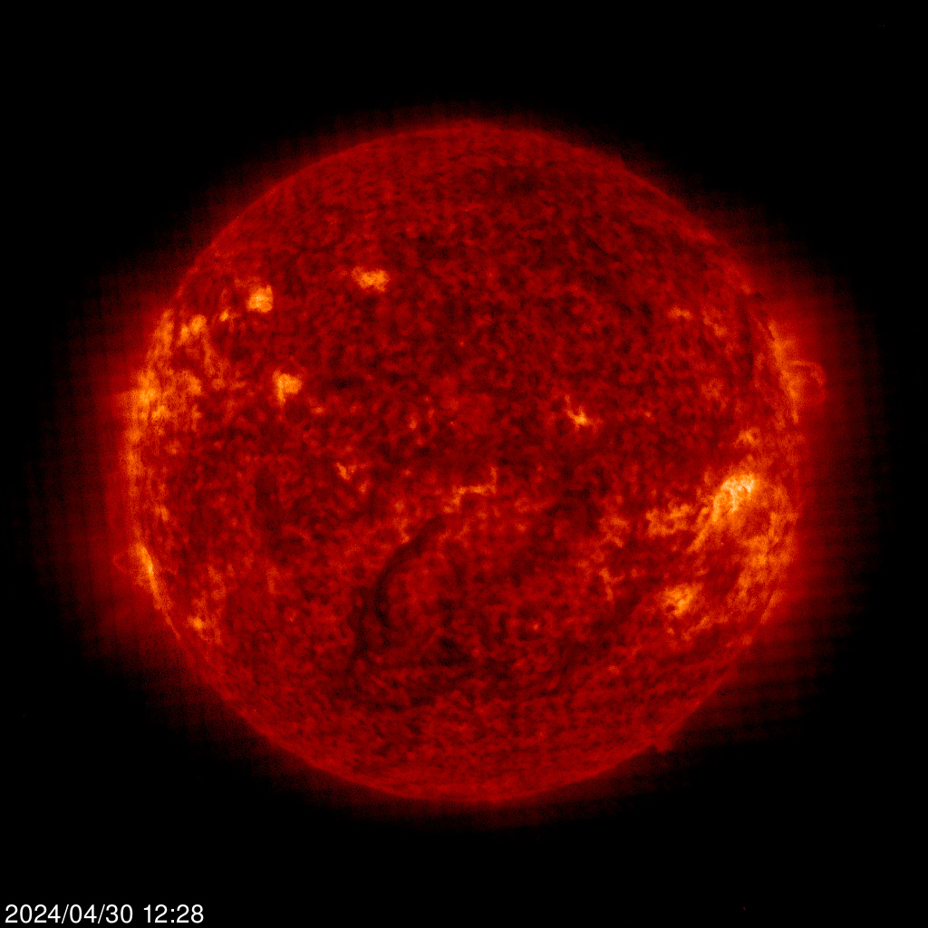
Pictures of the Sun taken by the SOHO's Extreme Ultraviolet Imaging Telescope (EIT), at different wavelenghts. Solar Data Analysis Center, NASA Goddard Space Flight Center. Click on each pìcture to see the high resolution version. Source: SOHO/NASA-ESA.
|
|
|
|
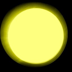
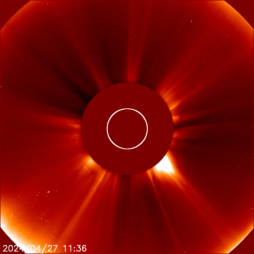
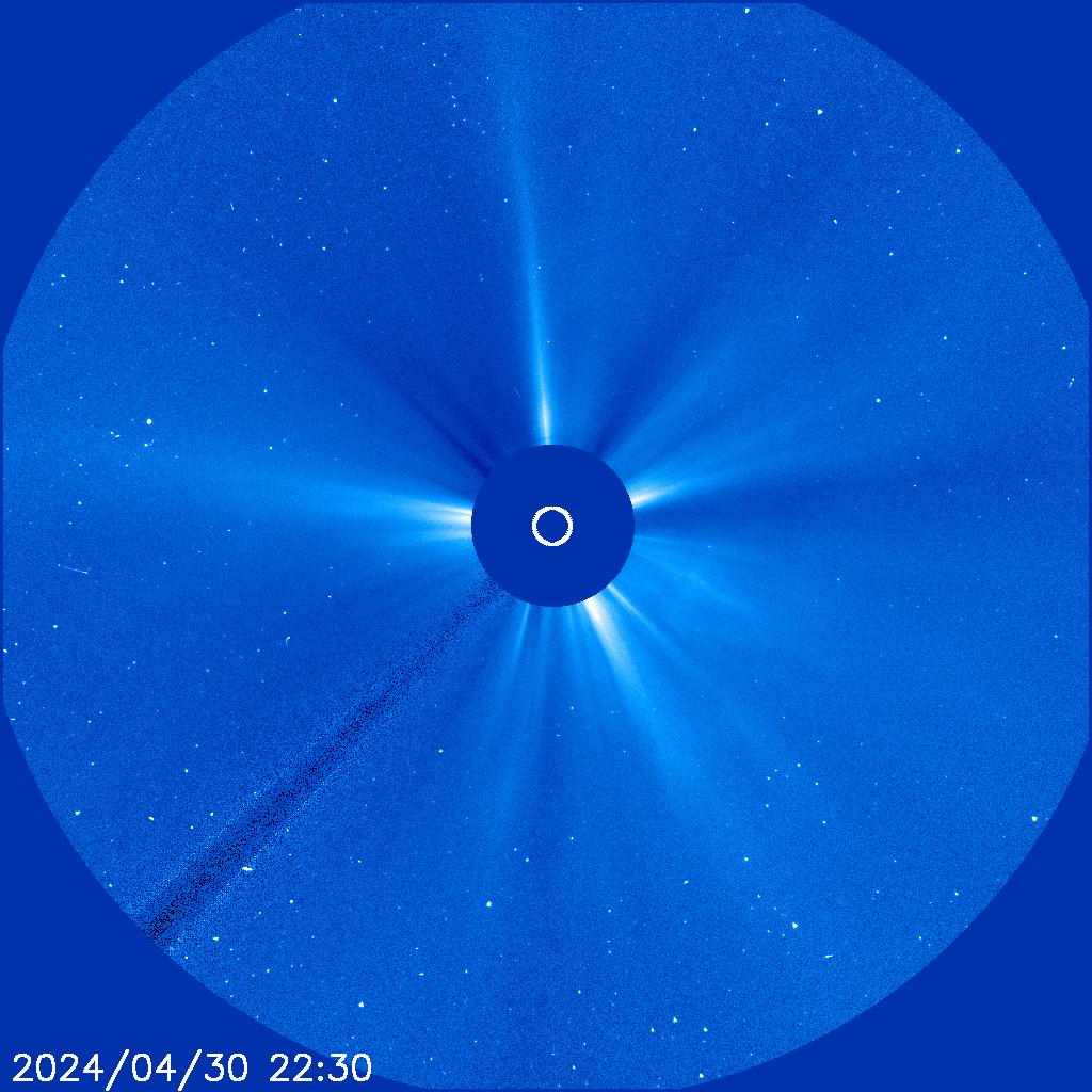
Images of the Sun taken by the SOHO's Large Angle Spectrometric Coronagraph (LASCO). C2 images show the inner solar corona up to 8.4 million kilometers (5.25 million miles) away from the Sun. C3 images show the outer solar corona up to 45 million kilometers (30 million miles) away from the Sun. Thanks to The coronagraphs, we are able to see the greatest solar flares and coronal mass ejections (CME) from the Sun. Click on each pìcture to see the high resolution version. Source: SOHO/NASA-ESA.
|
|
Coronameter image from the Mauna Loa Solar Observatory (Hawaii). The coronameter shows a clear view of the solar flares generating solar wind at very high speed.

Source: Mauna Loa Solar Observatory
Solar Activity
Solar Flux Index and Sunspots
Emission from the Sun at centimetric (radio) wavelength is due primarily to coronal plasma trapped in the magnetic fields overlying active regions. There is a direct relationship between the solar activity level and this emission, measured through the Solar Flux Index (SFI or F10.7). The SFI is a measure of the solar radio flux per unit frequency at a wavelength of 10.7 cm (2800 MHz). High values of SFI cause propagation openings in the higher HF bands.
Source: NOAA/N0NBH
The plots show the trend of the following parameters during the last month:
- Green plot: proton flux measured at the line He II 30.4 nm (NASA SDO EVE).
- Blue plot: proton flux measured at the line He II 30.4 nm (NASA SOHO CELIAS SEM).
- Red plot: SFI measured by the Dominion Radio Astrophysical Observatory (Canada).
- Yellow plot: sunspot number (SN) measured by the Boulder Observatory (NOAA), Wolf number.
The SFI value is updated every day at 21:00 from the NOAA's WWV station.
Another way to check the activity of the Sun at a given instant is by means of quantifying the Sunspot Number (SSN), a process which can be performed following different methods. The sunspots are solar regions radiating approximately half the energy of the rest of regions in the solar surface. The higher number of sunspots, the higher grade of ionization, causing the MUF to increase and making easier to establish ionospheric reflection radio communications in the higher HF bands. There is a strong correlation between the SFI and the SSN.

Source: SOHO/NASA
The image shows the latest picture taken with the SOHO's MDI instrument, where the current sunspots and sunspot groups can be seen. During the solar cycle minimums the sunspot number is very small, to the point that in some cases there are no sunspots at all. Every solar cycle can be identified by the magnetic polarity of their sunspots: for a given solar hemisphere (North or South), all the sunpots have the same polarity during the cycle. The sunspots in the other hemisphere will have the opposite polarity during the same cycle. Every 11 years, when one cycle finishes and the next one begins, the Sun flips its magnetic polarity and the orientation of the sunspots is also inverted.
The Mount Wilson Observatory in California provides the following sunspot classification:
| Type | |
| Alpha | A unipolar sunspot group |
| Beta | A sunspot group having both positive and negative magnetic polarities (bipolar), with a simple and distinct division between the polarities |
| Gamma | A complex active region in which the positive and negative polarities are so irregularly distributed as to prevent classification as a bipolar group |
| Beta-Gamma | A sunspot group that is bipolar but which is sufficiently complex that no single, continuous line can be drawn between spots of opposite polarities |
| Delta | A qualifier to magnetic classes indicating that umbrae separated by less than 2 degrees within one penumbra have opposite polarity |
| Beta-Delta | A sunspot group of general beta magnetic classification but containing one (or more) delta spot(s) |
| Beta-Gamma-Delta | A sunspot group of beta-gamma magnetic classification but containing one (or more) delta spot(s) |
| Gamma-Delta | A sunspot group of gamma magnetic classification but containing one (or more) delta spot(s) |
The sunspot number is necessary as a parameter for many HF propagation calculators and can be presented in a variety of formats. A link to the NOAAA's National Geophysical Data Center (NGDC) pages follows, where you can get current data about the Sunspot Number in different formats, including ISN (International Sunspot Number, compiled by the Sunspot Index Data Center in Belgium), American Relative Sunspot Numbers, ancient sunspot data and Group Sunspot Numbers.
Remark for VOACAP users: please use the following values, corresponding to the Smoothed International Sunspot Number (courtesy SIDC, Royal Observatory of Belgium):
2025 07  2025.538 :  121.0     0
2025 08  2025.623 :  116.7     0
2025 09  2025.705 :  113.1     0
2025 10  2025.790 :  113.9   6.6
2025 11  2025.873 :  111.1   7.1
2025 12  2025.958 :  112.4   7.9
2026 01  2026.042 :  110.5   9.1
2026 02  2026.122 :  108.2  10.0
2026 03  2026.204 :  105.3  10.7
2026 04  2026.286 :  101.8  11.2
2026 05  2026.371 :   98.3  11.7
2026 06  2026.453 :   94.5  12.0
2026 07  2026.538 :   91.0  12.3
2026 08  2026.623 :   88.0  12.6
2026 09  2026.705 :   85.4  13.0
2026 10  2026.790 :   82.7  13.2
2026 11  2026.873 :   79.9  13.3
2026 12  2026.958 :   76.9  13.3
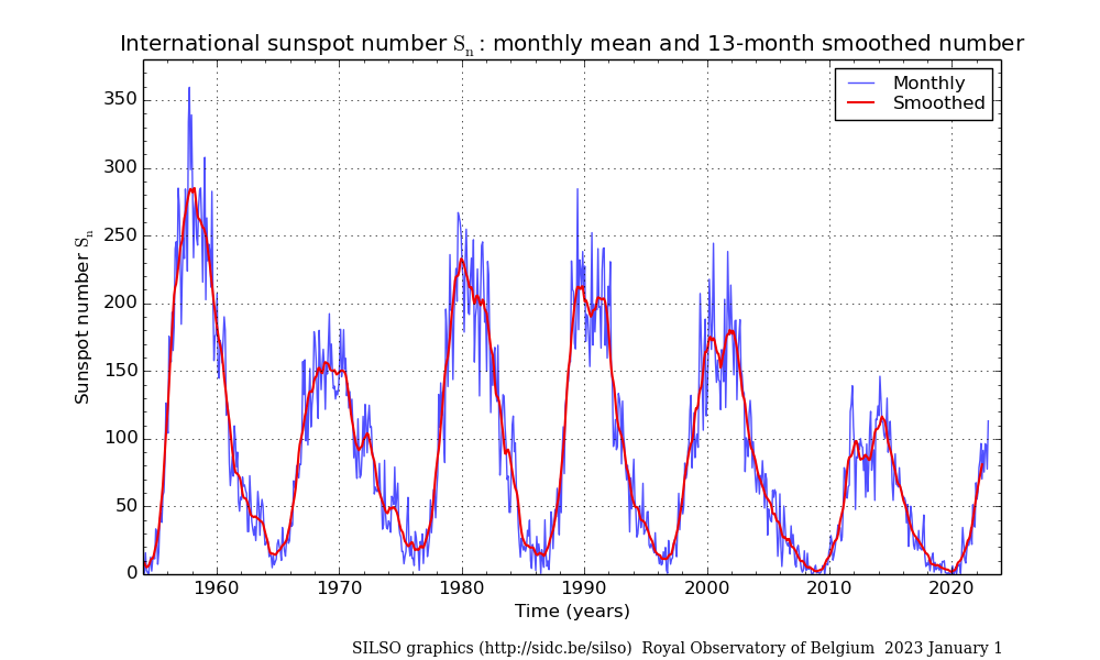
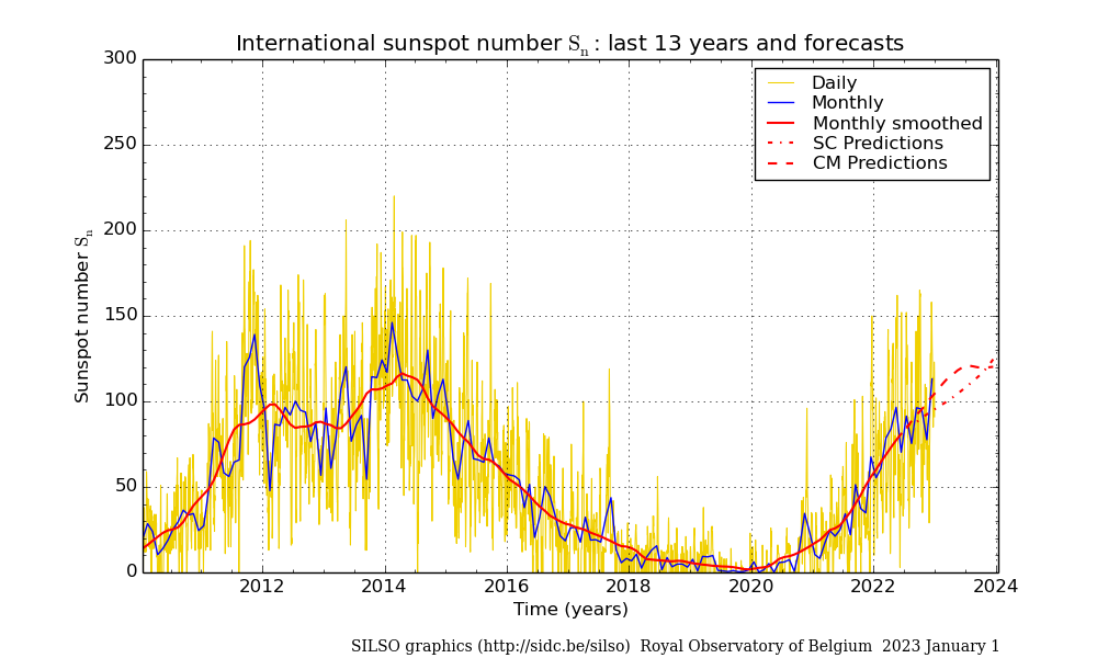
Source: SIDC, Royal Observatory of Belgium
The plots show the sunspot number evolution during the last years. This number follows periodic cycles of an estimated duration of 11 years. At the cycle peaks the sunspot number is higher and the propagation conditions improve. Due to the fact that some sunspots may appear grouped, the "Wolf number" is used in the computation, taking into account both the groups and the isolated sunspots. We are currently at solar cycle 25.
Sun-Earth Interaction
Solar Wind and Interplanetary Magnetic Field | Magnetopause Status
Solar Wind and Interplanetary Magnetic Field
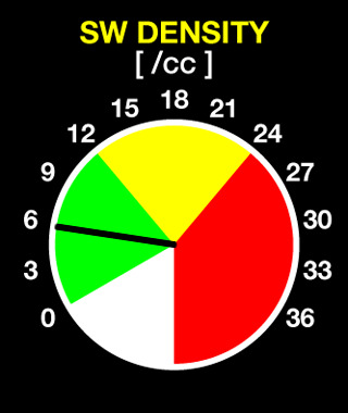
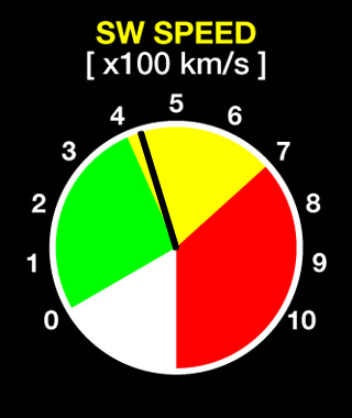
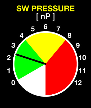
The solar wind is composed of electrically charged particles originated by solar flares, travelling at very high speed towards the Earth. Although the magnetosphere works as a protective shield for the Earth, in the event of very intense solar flares part of this wind hits the upper ionosphere, affecting radiocommunications in the HF and satellite bands.
Source: NASA/NOAA - ACE spacecraft
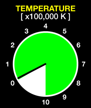
Last 6 hours data of the following solar wind parameters: Temperature (ºK), speed (km/s), proton density (protons/cm3), angle between the IMF vector and the YZ plane in GSM coordinates (Phi, degrees) and Interplanetary Magnetic Field magnitudes (Bt, Bz). Please take a look here for further information.
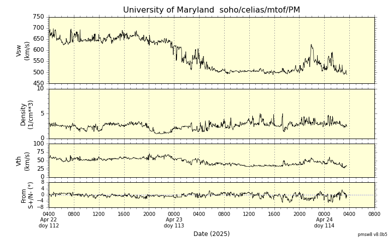
Source: Maryland University - SOHO Spacecraft
The Interplanetary Magnetic Field (IMF) is the name of the magnetic field created by the Sun. Due to the solar rotation (one complete rotation every 27 terrestrial days), it has an spiral shape. The Earth creates its own geomagnetic field, which works a a defensive shield against the solar wind and spreads through a region called magnetosphere. The region of the space in wich both magnetic fields interact is called magnetopause. If the IMF reaches the Earth following the southward direction, it can to a certain point cancel the Earth's magnetic field, making easier for the solar wind to reach the ionosphere and causing aurorae and geomagnetic storms.
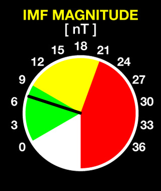
Source: Australian Space Weather Alert System - DSCOVR probe
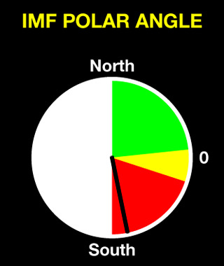
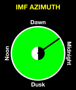
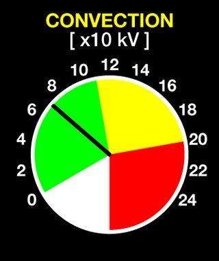
The IMF is a vectorial field wich three dimensions named x, y, z, the yz plane being orthogonal to the plane of the ecliptic. Following this coordinate system, if the Bz component of the IMF is negative, then the IMF points towards the South of the Earth and, if it is powerful enough, it can cause a geomagnetic storm. The plots show the angle of arrival ("clock angle") of the interplanetary magnetic field and it's intensity ("clock hand"). The plot changes to red when the IMF points towards the south and the intensity reaches at least 15 nT, thus providing a warning of possible geomagnetic storm conditions.
Angle ("clock angle") in degrees:
Angle = 0 --- IMF Bz north
Angle = 90 --- IMF By +ve
Angle = 180 --- IMF Bz south
Angle = 270 --- IMF By -ve
Sun-Earth Interaction
Magnetopause status
The magnetopause is the separation interface between the magnetosphere and the interplanetary space. It is normally located at a distance of about 10 times the Earth's radius, towards the Sun. However, during high solar activity episodes, this distance may be reduced to about 6,6 times the Earth's radius.

Source: SWPC / University of Michigan Geospace Model
In both figures, the Earth is in the center, being illuminated from the left by the Sun (not shown). In the left figure, we are looking down upon the North pole; thus the figure represents the equatorial plane. The figure on the right depicts the scene in a perpendicular plane. The solar wind flowing from the Sun is super-magnetosonic with respect to the Earth, causing the formation of a shock wave. As the solar wind flows through the shock, it is slowed down, and it's pressure is balanced by the pressure from the Earth's magnetic field. The boundary at which this pressure balance is achieved is called the magnetopause.
![]() Australian Space Weather Alert System: Magnetopause Model.
Australian Space Weather Alert System: Magnetopause Model.
Solar Radiation Storms
The Solar Proton Events (SPE) are originated when the protons emitted by the Sun are accelerated in its proximity after a solar flare, or in distant regions as an effect of the shock wave caused by a coronal mass ejection (CME). Those protons reach high energetic levels and after hitting the Earth can cause solar radiation storms. Those storms are originated between 15 minutes and several hours after a severe solar event and may have a duration of hours or even days, causing possible biological risks and affecting the satellite operations, radio communications and radionavigation systems.
In the HF band, attenuation levels of 1-4 dB each 1000 km may be reached. The attenuation can be extremely severe in transpolar radio paths, causing Polar Cap Absoprtion (PCA) events. If a solar radiation storm occurs, please check the HF Absorption Levels.
Solar Radiation Storms
Solar Proton Events (SPE) Monitors
The intensity of the solar radiation storms is quantified as a function of the measurement of the flux of particles (ions) with an energetic level greater that 10 MeV, coming from the Sun and originated in a SPE.
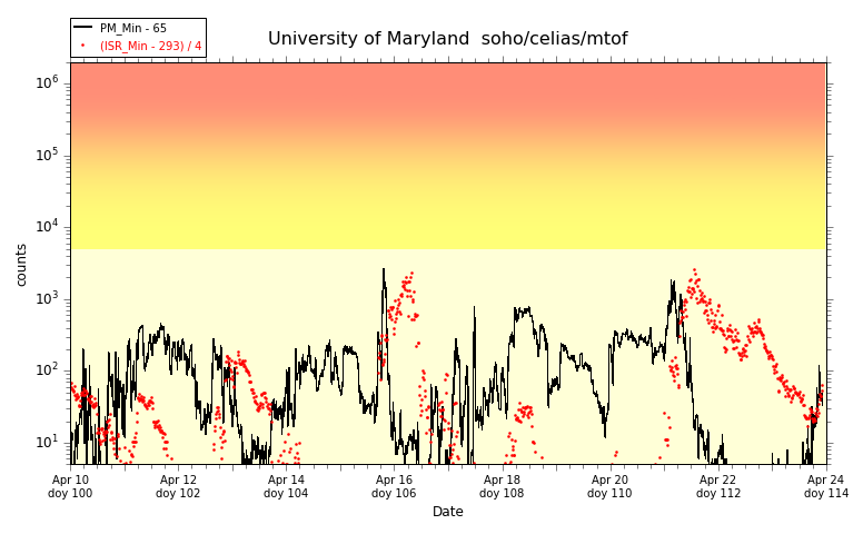
Source: University of Maryland - SOHO CELIAS/MTOF
The monitor shows the amount of energetic particles, according to the PM_Min formula. The solar wind with very high density or temperature can cause high values of PM_Min. However, it is considered that only values higher than 6000 are related to solar flares. In normal conditions (quiet solar wind), the values are under 100. The values higher than 100 indicate that a solar radiation storm is in progress.
Source: NOAA/SWPC - ACE spacecraft
The plots show the measured proton and electron densities for each energetic range between 35 and 1900 MeV. All values increase during solar radiation storms. ACE RTWS EPAM stands for "Advanced Composition Explorer Real Time Solar Wind Energetic Ions and Electrons".
Geomagnetic Storms
Kp Index | Ap Index | Dst Index
One to four days after a solar flare or a coronal mass ejection, a cloud of solar materials and their associated interplanetary magnetic field reach the Earth, saturating the ionosphere and causing a geomagnetic storm, which changes the magnetosphere and the ionosphere normal conditions. The effect is more intense in the equatorial regions and above 10 MHz, lasting hours (medium latitudes) or even 10-20 days (high latitudes). The geomagnetic storms are more frequent during periods of high solar activity, mostly after coronal mass ejections (CME). The radio waves of some frequencies may be subject to high absorption levels, causing fast fading events and uncommon radio paths.
There are two possibilities regarding radiocommunications: negative MUF variations (closing the higher bands in HF) and positive MUF variations (causing range extension in VHF). In addition to this, the HF absorption levels are higher, above all in the lower bands, so both events may cause a complete fadeout in HF. In case of a geomagnetic storm, please check the HF Absorption Levels and the foF2 variations due to geomagnetic activity. If you are a user of NVIS communications, it is interesting to check also the last available Ionograms.
Geomagnetic Storms
Kp Index
The geomagnetic field (the Earth's magnetic field) is perturbed due to its interaction with the Sun's Interplanetary Magnetic Field (IMF). Those perturbations can be measured using magnetometers, installed all along the Earth, wich offer the 'K indices' as a result of their measurements. The combination of the K indices measured by different magnetometers every 3 hours results in the 'Kp planetary index', which is represented in the following plot from NOAA.

Source: NOAA/SWPC
The following table shows the relationship between the Kp index, the Ap index (see next section) and the NOAA G-Scales. A brief description of each level is provided.
| Kp | Ap | NOAA | Status |
| Kp = 0 | 0 | No storm | Inactive geomagnetic field |
| Kp = 1 | 3 | No storm | Very quiet geomagnetic field |
| Kp = 2 | 7 | No storm | Quiet geomagnetic field |
| Kp = 3 | 15 | No storm | Unsettled geomagnetic field |
| Kp = 4 | 27 | No storm | Active geomagnetic field |
| Kp = 5 | 48 | G1 | Minor geomagnetic storm |
| Kp = 6 | 80 | G2 | Major geomagnetic storm |
| Kp = 7 | 140 | G3 | Severe geomagnetic storm |
| Kp = 8 | 240 | G4 | Very severe geomagnetic storm |
| Kp = 9 | 400 | G5 | Extremely severe geomagnetic storm |
Geomagnetic Storms
Ap Index
The geomagnetic field perturbations can be measured also using a similar parameter known as Ap planetary index. The following graph shows the near-real-time Ap planetary index computed by the Australian Space Weather Alert System:
Source: Australian Space Weather Alert System
The following table shows the meaning of the values:
| Ap | Status |
| 0 < Ap < 30 | Quiet geomagnetic field |
| 30 < Ap < 50 | Minor geomagnetic storm |
| 50 < Ap < 100 | Major geomagnetic storm |
| Ap > 100 | Severe geomagnetic storm |
Ionosphere status
Grade of ionization (TEC Maps)
Grade of Ionization (TEC Maps)
The Total Electron Content (TEC) gives an idea about the ionization grade of the ionosphere. Its unit of measurement is the TECU (1 TECU = 10E+16 electrons per square meter). The zones with the highest TEC are affected by the occurence of different ionization phenomena, such as photoionization, absorption, etc.
Source: Australian Space Weather Alert System (IRI-90 ionospheric model)
Source: Jet Propulsion Laboratory (JPL)

Source: IMPC/DLR (Germany)
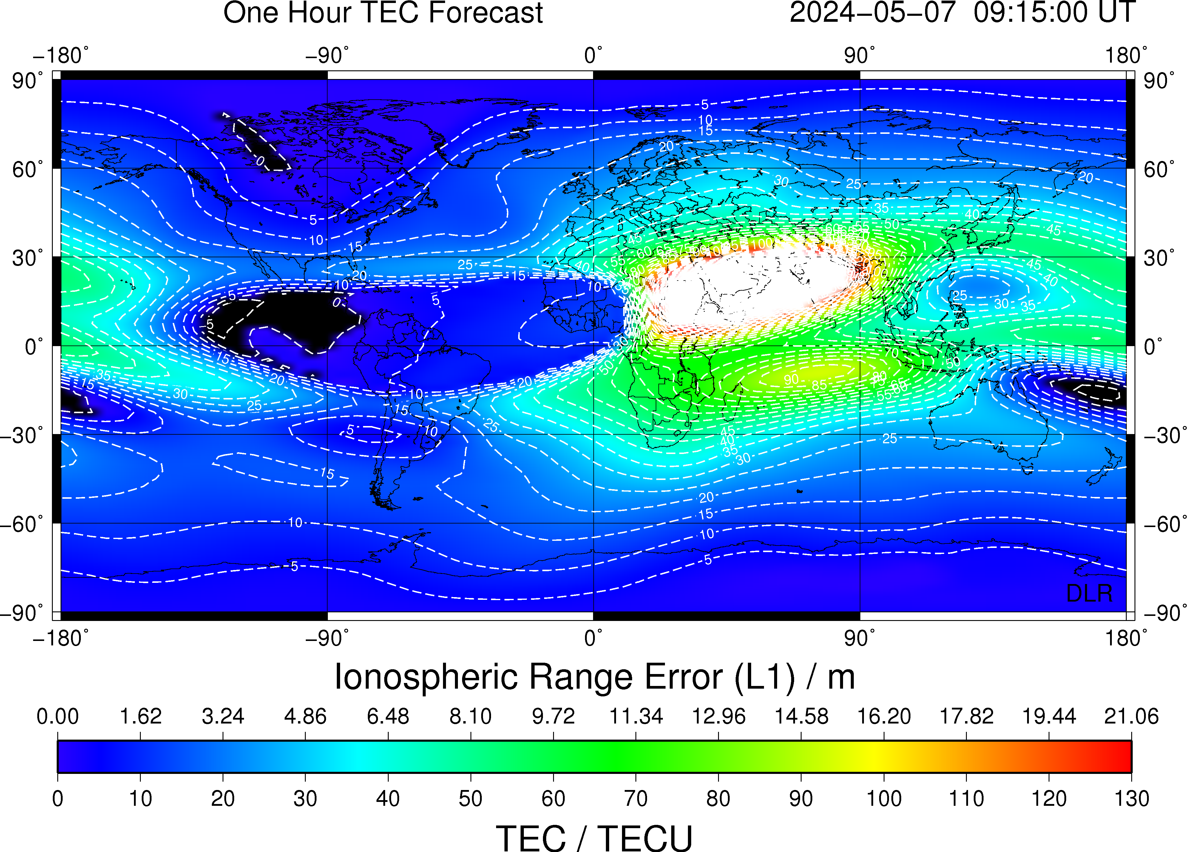
Source: IMPC/DLR (Germany)
The maps are colored by total electron content. The warmest colors represent the higher TEC values, i.e. within regions of direct solar incidence (photoionization). As a general rule, the F2 layer cut frequency (foF2) will be higher with a great TEC. This way, those maps can give an idea of the hours of the day in which the foF2 is expected to be low or high. The maps are derived from measurements of the carriers of the GPS.
Radiocommunications
Spectrum Monitors | HF Absorption | Ionograms | foF2 | foF2 Variations | MUF(3000) | MUF Calculators | Grey Line | HF Optimal Working Frequencies
|
|
|
|
|
| HF Comms Warning | Current HF Fadeoutl | HF Fadeout Warning | Polar Absorption (PCA) | |
Source: Australian Space Weather Alert System |
||||
Radiocommunications
Spectrum Monitors
During a solar flare event, intense electromagnetic radiation in the X-Rays band and the radio bands is emitted from the Sun. When this radiation reaches the Earth, a noise storm may occur, making worse the signal-to-noise ratio in radiocommunication systems working in the HF, VHF and UHF bands. The noise storms usually last from minutes up to one hour, although a chain of events may last even more. The spectrum monitors allow us to analyze the intensity of the radio signals received in a particular radiocommunications band, showing the results in graphical diagrams. Those measurements provide an idea of the better working frequencies for each hour of the day.

Source: NICT/Hiraiso Solar Observatory

Source:Humain Radioastronomy Station, Royal Observatory of Belgium
Source: SIDC
The images show several spectrum monitors in the VHF and UHF bands, placed in Australia, Japan and Belgium. Please take into account that noise storms affect the sunlit areas of the Earth (day), so during the local night those instruments do not detect any storm. During a solar flare, check the sunlit areas using the Grey Line map.
Radiocommunications
HF Absorption
During or after a solar flare, the X-ray emissions, the solar radiation storms and the geomagnetic storms may cause a rise of the grade of ionization in the D-layer of the ionosphere, increasing the absorption of the radio waves travelling through this layer up to levels that may be of importance. As a result, fading in the HF radio links may occur, especially in the lower frequencies of the band.
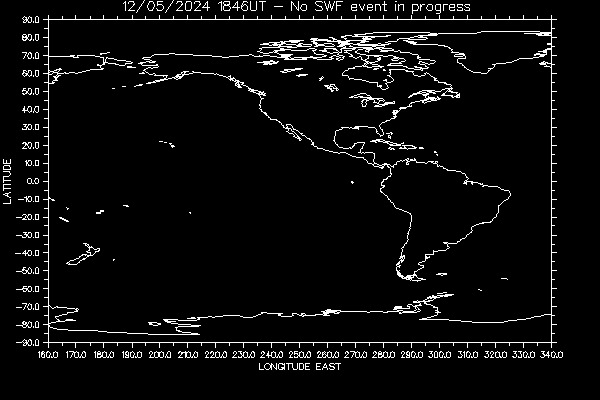
Source: Australian Space Weather Alert System
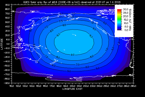
Source: Australian Space Weather Alert System
The maps show the Absorption Limited Frequency (ALF), that is, the minimum frequency able to propagate along about 1500 km paths during absorption events. To interpret the map during one of those events, estimate the first reflection point in the ionosphere for the working path and identify the ALF using the contour lines. If the frequency of operation is lower than this estimated ALF, it is most probably that the radio link will not work. Using a frequency of operation (if possible, depending on the MUF) higher than the ALF increases the probability of establising the radio link. The first map shows real time data and the second map shows the ALF during the last important event (check the date).
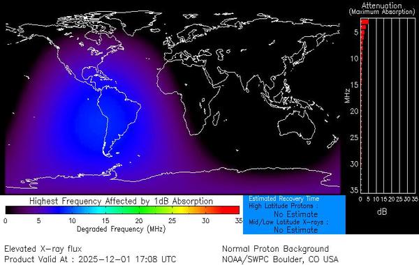
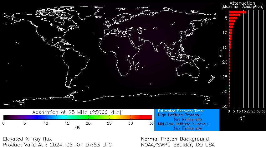
Source: NOAA/SWPC - DRAP2
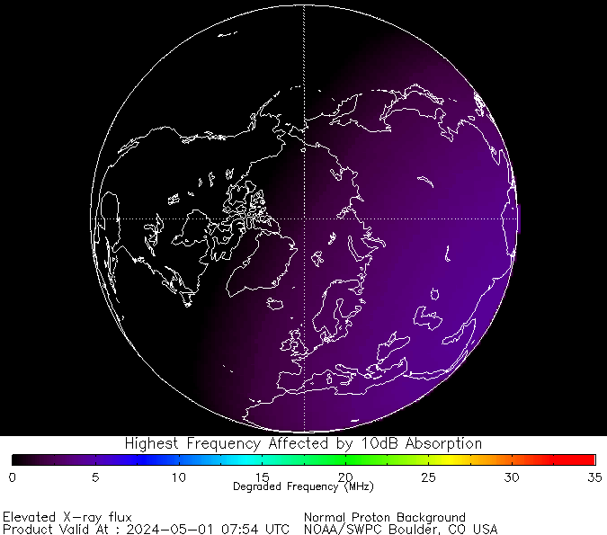 North Pole radio paths Source: NOAA/SWPC - DRAP2 |
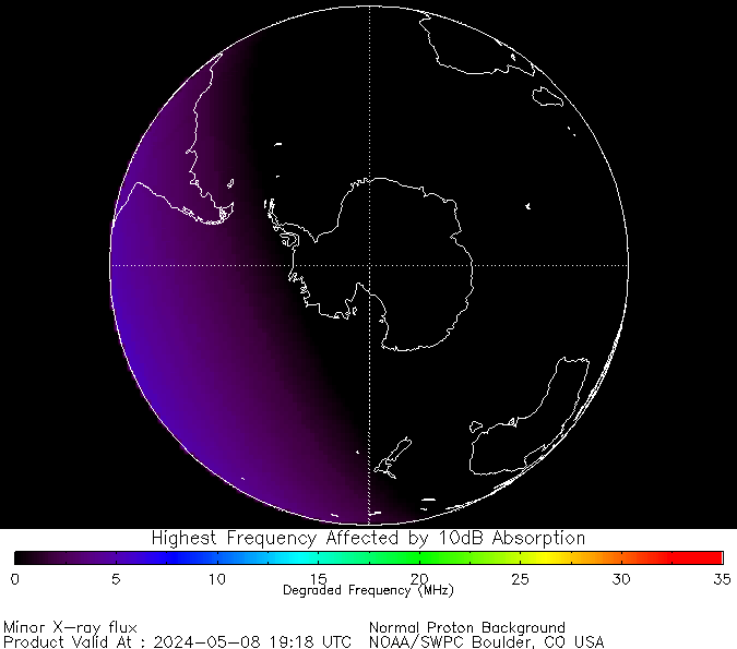 South Pole radio paths Source: NOAA/SWPC - DRAP2 |
 |
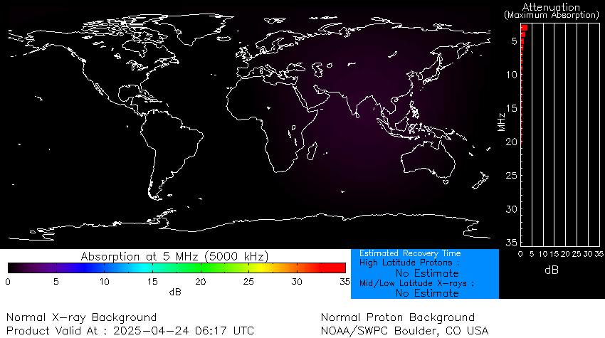
The maps provided by NOAA show the highest affected frequency (HAF) by 1 dB absoprtion (world map) or 10 dB (polar area maps), for vertical radio paths. Radio links working in frequencies lower than the HAF will be affected by higher absorption values In the world map, the attenuation bar graph on the right-hand side of the graphic displays the expected attenuation in dB as a function of frequency for vertical radio wave propagation at the point of maximum absorption on the globe. This graph is only valid at this point. In order to compute the resulting total approximate absorption for HF circuits in other areas and frequencies, please use the following procedure:
1) Make an estimate of the coordinates of the first point of ionospheric reflection for your HF circuit.
2) Check the NOAA DRAP2 tabular values and pick the HAF for this point. At this frequency, the absorption level is:
A(HAF) = 1 dB
3) Compute the absorption for your frequency of operation "F", using the following formula:
A(Fver) = (HAF/F)^(3/2) x A(HAF) = (HAF/F)^(3/2) dB
4) If "T" is the takeoff angle of your antenna, the absorption for the corresponding oblique path at the same point is:
A(Fob) = A(Fver)/sin(T) dB
5) Repeat the procedure for all ionospheric reflections in the radio path and finally add up all the computed absorptions.
 Source: NOAA/SWPC - DRAP2 |
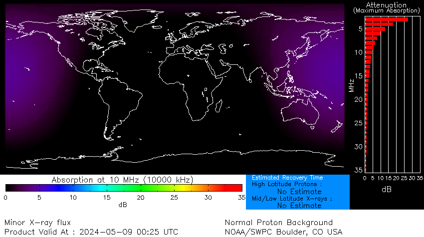 Source: NOAA/SWPC - DRAP2 |
 Source: NOAA/SWPC - DRAP2 |
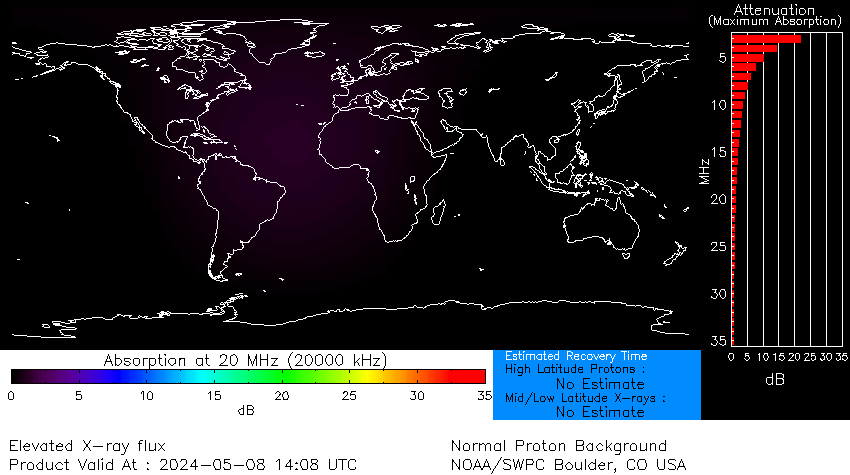 Source: NOAA/SWPC - DRAP2 |
 Source: NOAA/SWPC - DRAP2 |
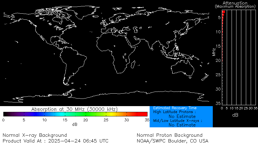 Source: NOAA/SWPC - DRAP2 |
he six maps shown above are provided by NOAA and show the global ionospheric D-Region absorption prediction at 5, 10, 15, 20, 25 and 30 MHz for vertical radio paths (NVIS). If "T" is the takeoff angle of your antenna, the absorption for the corresponding oblique path at the same point is:
A(Fob) = A(Fver)/sin(T) dB
Being A(Fver) the absorption observed in the map for the vertical radio path and A(Fob) the absorption calculated for the oblique path. Please take into account that each map is valid only for the specified frequency.
Radiocommunications
Ionograms
If the radio wave reaches the ionosphere following a vertical o near vertical path (NVIS), reflection will occur in the F2 layer only if the frequency of operation is below a threshold known as F2 layer critical or cut frequency (foF2), which can be measured using ionosondes. Two ionosondes provide public data in Spain: The Ebro Observatory (Roquetes, Tarragona, NE) and the National Institute for Aerospace Technology (El Arenosillo, Huelva, SW). The corresponding latest ionograms are shown. If you look for data from other ionosondes around the world, please see the world map below.
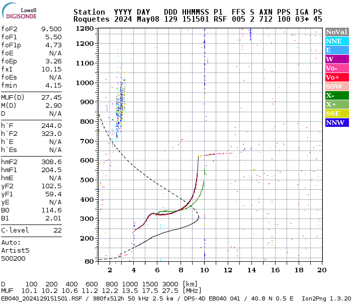
Source: Ebre Observatory
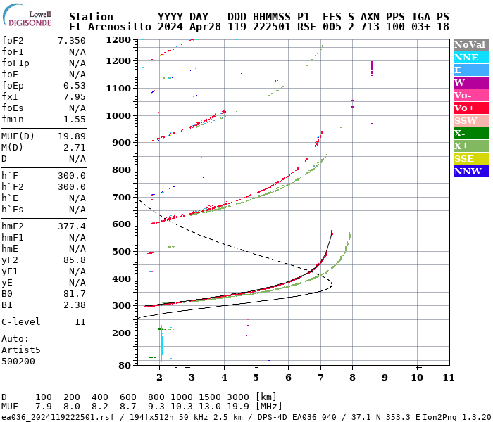
Source: Spanish National Institute for Aerospace Technology (INTA)
The intepretation of all the data collected by an ionosonde is a quite difficult process. Frequency (MHz) is represented on the X-axis and the virtual height (km) on the Y-axis. If the ionosonde detects ionospheric reflection for a particular frequency, a point is drawn on the coordinates corresponding to that frequency and virtual height. On the left side we can find derived empiric data such as the measured critical frequency foF2 (MHz) and some estimated data such as the standard MUF for radio links of 3000 km (MUF(D)). On the bottom side we can find an estimation of the MUF derived for different distances, very useful if your goal is to establish HF radio links from points near the ionosonde to other stations located at the indicated distances, using oblique paths.
Source: Center for Atmospheric Research, University of Massachussets Lowell
Radiocommunications
foF2 Maps
If the radio wave reaches the ionosphere following a vertical o near vertical path (NVIS), reflection will occur in the F2 layer only if the frequency of operation is below a threshold known as F2 layer critical or cut frequency (foF2), which can be measured using ionosondes. The following experimental maps are built using data from ionosondes located in Australia, Japan, South Africa, Italy, Argentina and the United States.
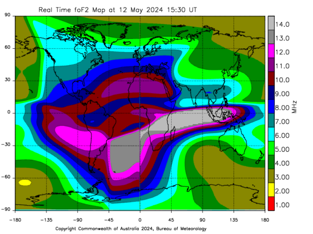
Source: Australian Space Weather Alert System
Each map shows an extrapolation of the foF2 derived for each region, using data from the nearest ionosondes. Those values can be used as MUF thresholds for NVIS (Near Vertical Incident Skywave) links, that is, using an aerial system with a very high takeoff angle, being able to reach ranges of up to 500 km without shadow areas.
Radiocommunications
foF2 variations due to geomagnetic activity
When the geomagnetic activity is high, as a consequence of geomagnetic storms started by solar flares or coronal mass ejections (CME), the F2 layer cut frequency foF2 may suffer important variations which could affect the HF radio links, both NVIS and long-distance. A geomagnetic storm may cause the ionosphere's grade of ionization to be increased (higher foF2 and MUFs) or diminished (lower foF2 and MUFs).
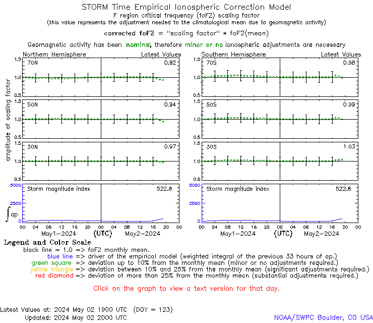
Source: NOAA/SWPC
This NOAA/SWPC graph shows the F region critical frequency (foF2) scaling factor, to be applied to the foF2 mean value in real-time during a geomagnetic storm. This graph provides an idea of the influence of a geomagnetic storm on the foF2 and the MUF. There are separate graphs for the Northern and Southern Hemispheres and for three latitude areas: 30º, 50º and 70º. Values equal to 1 are an indicator of normal conditions, that is, it is not necessary to apply corrections to the foF2 values. In order to get the exat value of foF2 in real time, check the ionograms available in this panel.
Radiocommunications
MUF(3000)
The URSI defines the MUF as "the maximum frequency for inospheric transmission using an oblique path, for a given system". Using oblique paths, we will have a different MUF for each link distance. The following map shows MUF data for radio links larger than 3000 km.

Source: K2CG (prop.kc2g.com)
The map has been developed by Andrew Rodland (K2CG), through the development of an open source project available at Github, which was presented at the HamSCI 2021 conference. It uses data from NOAA NCEI and GIRO. The numbers within circles represent the MUF(3000) directly computed by the corresponding ionosphere sounding stations. The MUF(3000) map for the remaining locations is then generated using interpolation. In order to determine the estimated MUF for a radio link, using this map:
3000 km PATHS: Estimate where the path midpoint is located and determine the corresponding frequency using the color scale.
4000 km PATHS: Estimate where the path midpoint is located and determine the corresponding frequency using the color scale. Multiply this value by 1.1.
PATHS LONGER THAN 4000 km: Split the path into 3000 km or 4000 km equal-lenght segments (choose the alternative that provides a better adjustment). Choose the two segments at the edges of the path and compute the MUF for each one, using the methods described above. The complete path MUF will be the lower value of these two figures.
Radiocommunications
Online MUF Calculators
Free online software available on the Internet for MUF calculations using a variety of parameters.
VOACAP Online |
Prediction Online Tools |
Radiocommunications
Grey Line
The grey line is the da/night terminator line over the Earth. The D Region in the ionosphere (where HF signals absorption occurs) quickly disappears in the dark side of the grey line, rising again in the opposite side. Propagation conditions will be enhanced for radio paths following the grey line.
Source: Fourmilab Earth and Moon Viewer
The figure shows the position of the grey line (day/night terminator) in the world map. This map is also interesting to identify the geographical areas potentially affected by solar events hitting the day area of the Earth, such as the radio fadeouts caused by X-Ray emissions, or the noise storms, which can be analyzed with the help of spectrum monitors.
Radiocommunications
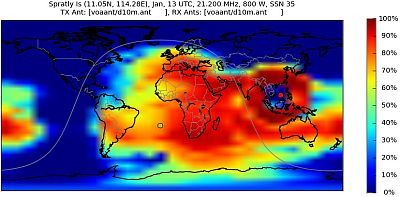
HF Optimal Working Frequencies
Current optimal working frequencies for global radio links. Reliable during 80% of time of the corresponding month, unless there is an occurrence of events related to space weather: radio fadeouts, solar radiation storms and geomagnetic storms.
Source: Propagation Resource Center - NW7US (HFRadio.org)
Select the region where your HF transmitter is located. You will get a table with the optimal working frequencies to establish radio links with all the other areas.
Aurora
Aurora Forecasts
Aurorae borealis occur during episodes upon which the interplanetary magnetic field (IMF) module is powerful enough and its Bz component points southwards when reaching the Earth. The solar wind reaches the polar areas and collides with the atoms and molecules of the upper layers of the atmosphere, causing the emission of radiation at different wavelengths (colors). Aurorae borealis activity causes the electric currents within the ionosphere to increase, making higher the probability of fading in the radio paths crossing the aurora due to absorption, especially in the 160 meters HF band.
Aurora Forecasts
Aurorae borealis occur during episodes upon which the interplanetary magnetic field (IMF) module is powerful enough and its Bz component points southwards when reaching the Earth. The solar wind reaches the polar areas and collides with the atoms and molecules of the upper layers of the atmosphere, causing the emission of radiation at different wavelengths (colors).
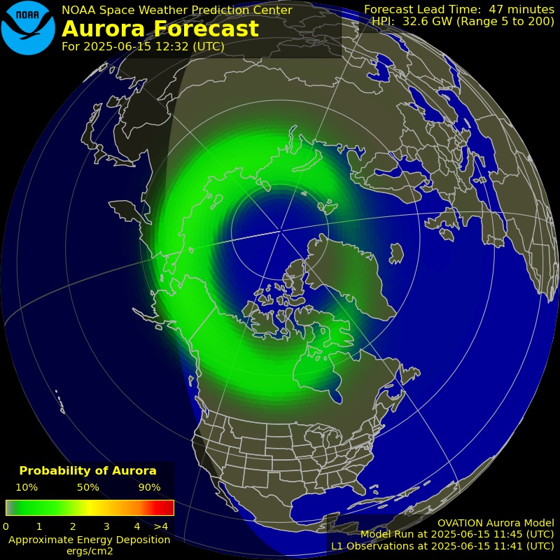
Source: OVATION Auroral Forecast (NOAA)
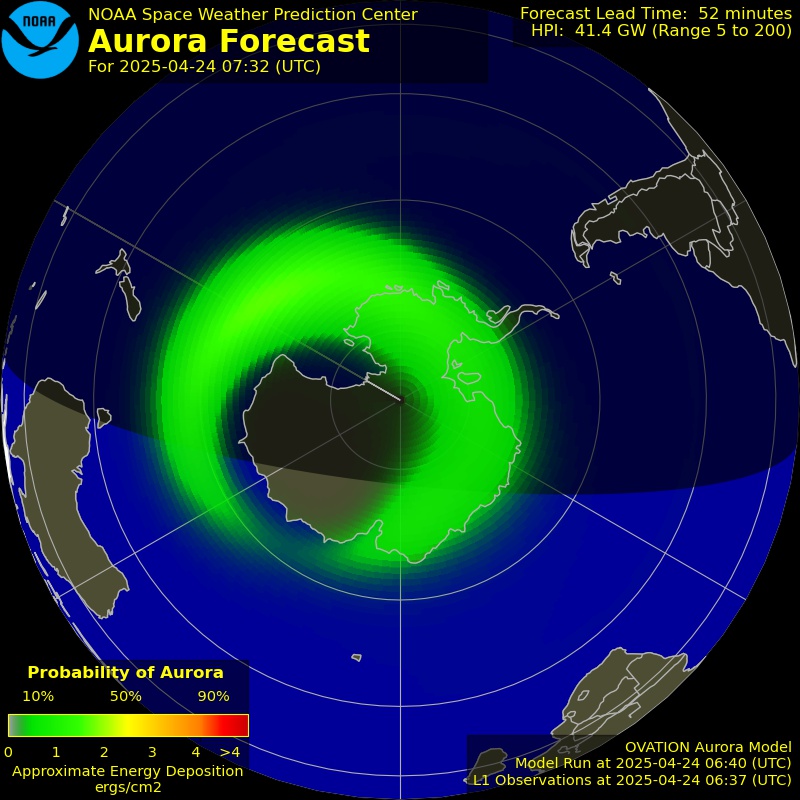
Source: OVATION Auroral Forecast (NOAA)
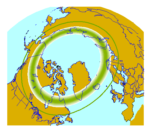
Source: Geophysical Institute, University of Alaska Fairbanks
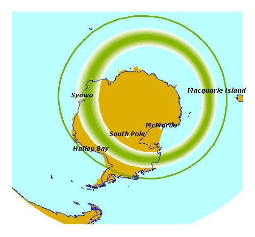
Source: Geophysical Institute, University of Alaska Fairbanks
External Links
PREDICTION AND OBSERVATION CENTERS | INTEGRATED TOOLS | REPORTS | FORECASTS | SOLAR ACTIVITY | GEOMAGNETISM | AURORAE | RADIO COMMUNICATIONS | RESEARCH AND EDUCATION
Prediction and Observation Centers
Integrated Tools
| Integrated Space Weather Analysis System (ISWA) | |
| RayTRIX Oblique Trace Synthesizer (UMASS Lowell) |
Reports & Data Repositories
Forecasts
| Space Weather Advisory Outlook (SWPC) | |
| Solar Conditions Summary and Forecast (Australian BOM) |
Solar Activity: Solar Cycle and Sunspots
| Solar Cycle Progression (SWPC) | |
| Datos Solares (Observatori de l'Ebre) |
Geomagnetism
Aurorae
| OVATION Live Display (Johns Hopkins Applied Physics Laboratory) | |
| AuroraWatch UK (Lancaster University) |
Radio Communications
Research and Education
This page is automatically reloaded every 15 minutes
Page last updated: 18 MAY 2022.
Main |
HF Central |
VHF-UHF Central |
Technical |
Follow @sn_4fu |


