Analysis of the radio contacts between the Canary Islands and South America in the 50 MHz band in March 2010

Main → Technical Articles → Analysis of the radio contacts between the Canary Islands and South America in the 50 MHz band in March 2010

Este artículo también está disponible en español (this article is also available in Spanish).

Abstract:

Analysis of the DX events in the 50 MHz band, between the Canary Islands, Brazil, Uruguay and Argentina, occured from 17th to 22nd March 2010 and the 1st April 2010. The radio links were of the transequatorial type, in the VHF band, with several peculiarities such as the wide angle of the radio path and the geomagnetic North-South direction, the lack of simmetry with respect to the geomagnetic equator or the poor conditions normally expected during the solar cycle minimum. Several hyphotesis are studied, such as the nE modes, the nF modes, complex modes or eTEP, through the analysis of ionospheric conditions, the approximate geometry of the link and the power budget. The analysis has not been finished yet. If you want to provide your comments or additional data, please use this form.

Table of contents.

1. Introduction.

2. Equatorial ionosphere characteristics.

2.1. Equatorial anomaly.

2.2. FAI and turbulences.

3. Technical information on the radio contacts.

3.1. Radio contact logs.

3.2. Statistical analysis.

3.3. Methodology used in the calculations.

4. Analysis of the ionospheric conditions.

4.1. Space weather conditions.

4.2. Total electron content (TEC).

4.3. Ionograms.

4.3.1.Tucumán ionosonde data.

4.3.2. Ascension Island ionosonde data.

4.3.3. Fortaleza ionosonde data.

4.3.4. Sao Luis ionosonde data.

4.3.5. Cachoeira Paulista ionosonde data.

4.4. Ionospheric scintillation maps.

5. Propagation modes hyphotesis.

5.1. One-hop hyphotesis.

5.2. 2F hyphotesis.

5.3. Complex modes hyphotesis.

5.4. eTEP hyphotesis.

5.5. 2E/3E/4E hyphotesis.

6. Conclusions.

7. References.

8. Glossary.

9. Acknowledgements.

1. Introduction.

This is an study about the radio contacts made by stations of the Amateur Radio Service between the Canary Islands (Spain) and several countries in South America, in the 50 MHz band, between the days 17 and 21 March 2010.The peculiarity of those contacts is due to:

The links are of the very long distance transequatorial type, in the VHF band.
They were made during the solar minimum (SSN=33), at the beginning of solar cycle 24, so low MUF values should be expected.
There was a very wide angle between the radio path and the geomagnetic North-South direction.
The circuits are not symmetric with respect to the geomagnetic Equator.

Using technical and scientific data available to the public, several hyphotesis about the possible propagation modes used are raised. For each case, the following aspects will be considered:

Analysis of the ionospheric conditions.
Approximate geometry of the radio link.
Power budget.

The first section is a summary of the available technical information about the radio links. An analysis about the ionospheric conditions during the days under study follows.

Later, several hyphotesis about the possible propagation modes are raised and a summary of the conclusions is offered. We will consider the following:

Propagation using only one of and equatorial scattering.
Propagation using two hops in the F2 layer of the ionosphere (2F).
Propagation by complex modes (1F1E/1E1F).
Evening eransequatorial propagation (eTEP).
Propagation using several hops in the E layer of the ionosphere (2E/3E/4E).

At the end of the article you will find a section about the references used and a glossary.

A great part of the opinions and data about those contacts have been provided by several spanish amateur radio operators, such as EA3EPH, EA5EF, EC7DND, EA8BPX, EA1DDO, EA8DD, EA6DX, EA6VQ and EA1FBF, via the Spanish Amateur Radio Union (URE) online forum.

Due to the fact that those contacts may be of some scientific interest on the matter of radio propagation studies, technical report have been sent to IPS Radio and Space Services, an institute managed by the Australian Government with a wide expertise on radio communications, and to the Ebro Observatory, in Spain.

2. Equatorial ionosphere characteristics.

The ionosphere is a non homogeneus medium presenting great differences with the latitude. We can distinguish three regions:

Polar ionosphere. Near the Earth's poles, the geomagnetig field lines are almost perpendicular to the Earth's surface, causing this zone to be more exposed to the effects of space weather. Common phenomenons in this region are aurorae and polar cap absorption events due to solar radiation storms and geomagnetic storms.
Template ionosphere. At medium latitudes, the different layers of the ionosphera have a more defined vertical structure.
Equatorial ionosphere. From the Equator to latitudes up to 20 degrees, the Sun is almost perpendicular to the Earth's surface and photoionization is at its maximum. Also, the geomagnetig field lines are parallel to the Earth's surface.

The equatorial ionosphere presents also other characteristics of interest, such as anomalies and irregularities, which will be described in the following sections.

2.1. Equatorial anomaly.

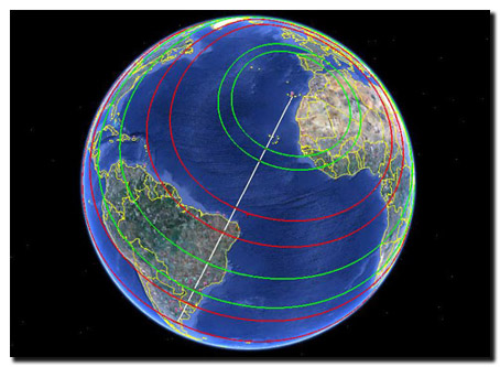
In the equatorial ionosphere, due to the fact that the Sun radiates in an orthogonal fashion over the Equator, it should be expected that the ionization maximums occur in this area. However, measurements show that those maximums occur at magnetic latitudes between 10º and 20º, phenomenon known as equatorial anomaly or Appleton anomaly. Let's remember also that the magnetic Equator and the geographic Equator have different locations.

The figure 2.1 shows an image of the total electron contect (TEC) of the ionosphere, the day 04/01/2010 at 17:45 GMT, obtained from the model Earth Space 4-D global 4-D ionosphere provided by Space Environment Technologies. The figure shows also the geomagnetic Equator position (orange line) and the radio path between the Canary Islands and Brazil (white line). The areas with warmest colors indicate an higher electron content. Pay attention to the fact that the maximums occur at both sides of the geomagnetic Equator.

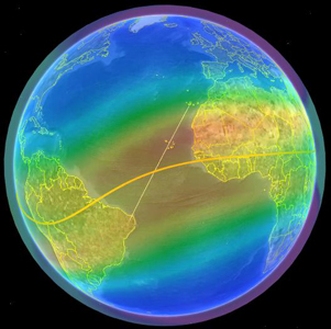
Fig 2.1. Equatorial anomaly (ES4D global ionosphere, Space Environment Technologies).

The regions with higher TEC will have also the highest values of foF2 (critical frequency of the F2 layer).

2.2. Turbulences and FAI.

Another characteristic of the equatorial ionosphere is the generation, around sunset, of turbulences shaped as bubbles, known as equatorial plasma bubbles (EPB), whose density of ionization is low compared to the surrounding areas [Ref.Harrison].

Those bubbles can be between 40 km and 350 km in diameter and are originated at the bottom part of the ionosphere, raising at speeds of 125-350 km/s to altitudes up to 1500 km. As the bubbles rise, they are aligned with the geomagnetic field (parallel to the Earth's surface in this region, as stated before), following the magnetic North-South lines. This is the reason they are called also field aligned irregularities (FAI), and can spread along the magnetic field line several thousand kilometers [Ref.Maruyama].

On the other hand, being composed of moving electrons, the bubbles are also affected by equatorial electrojet (EEJ), which drifts them eastwards at speeds between 25-125 m/s.

The figure 2.2 shows an orientative sketch of the evolution of this kind of ionospheric turbulences with time.

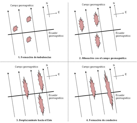
Fig 2.2. Formation of field aligned irregularities (FAI).

The figure 2.3 is an image taken by the NASA's TIMED (Thermosphere Ionosphere Mesosphere Energetics and Dynamics) spacecraft, where we can see the formation of EPBs in the equatorial area, aligned with the geomagnetic field.

Fig 2.3. Example of EPBs observed by the TIMED NASA's spacecraft.

The existing gradient of density of ionization between the inner part and the outer part of the bubbles causes the radioelectric waves travelling through them to be subject to refraction, scattering, diffraction and amplitude and phase variations, phenomenon known as scintillation, which may affect the satellite communication systems and also the HF/VHF radio links.

Those gradients may involve the formation of tubes or ducts which conduct the radio waves, allowing i.e. the propagation of VHF radio waves at long distances between both Earth's hemispheres (TEP, transequatorial propagation), as shown in the figure 2.4.

Fig 2.4. Formation of propagation ducts by the FAIs (E.R.Young et al, 1984).

The occurrence of those irregularities can be monitored using several methods, among them:

Range spread or spread-F in ionograms. The lines corresponding to each layer of the ionosphere are commonly well defined in an ionogram. However, if there is an irregularity near the ionosonde, those lines will spread vertically.
Scintillation maps. Scintillation is steadily monitored from several Earth stations because it can affect the satellite communication systems. Some agencies provide scintillation maps that we can use to locate ionospheric irregularities.

3. Technical information on the radio contacts.

In this section, the available technical information about the radio contacts is shown: dates, hours, stations contacted and their location. We discuss the azimuth-distance distribution, taking into account the locations of all the stations involved.

The methodology to calculate the theoretical fading margins is explained, considering also the technical data to calculate the power budgets. This data will be employed later for the validation of each hyphotesis.

3.1. Radio contact logs.

Several amateur radio stations in the Canary Islands (Spain) have reported to contact amateur radio stations in South America, especially in the north-east area of Brazil, using the 50 MHz band, between the days 18 and 21 March, 2010 and the 1st April, 2010.

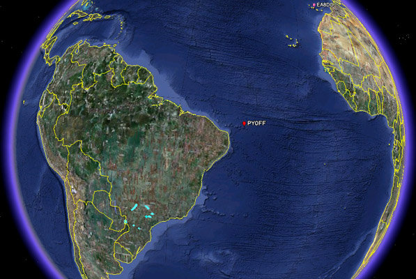
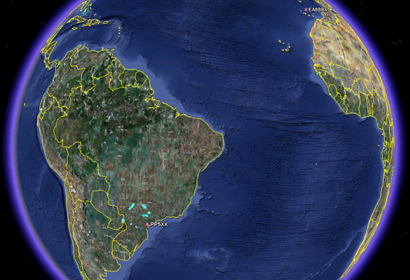
The figure 3.1. shows the representation in Google Earth of the locations of all the radio stations contacted. The kmz file is available for download: "EA8-PY_DX_50_MHz_Mar_2010.kmz".

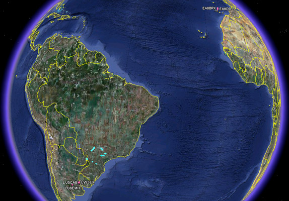Fig 3.1. Locations of all the stations involved in the contacts.
Click on each image to see a larger version

As we will see, in all the contacts registered the reported signal levels in the Canary Islands were high and the EA8 operators said that those signals kept at a steady level during the QSOs. Operators said also that they didn't notice neither signal fading nor frequency shifts during the contacts.

In the analysis, it is necessary to take into account the lack of information about the distribution of the population of amateur radio operators in the territory, especially in the theoretical areas of radio coverage. In example, when evaluating the multiple hop modes, it is possible that in some of the areas where radio coverage should exist, there aren't any contacts registered due to the fact that there aren't any amateur radio operators in the area or even that they weren't active at the hour and frequency of the band openings.

In some cases, the theoretical coverage areas for some of the hops lay in the Atlantic Ocean, where the probablity of having operative amateur radio stations is extremely low.

3.1.1. EA8BDD's log.

In the table 3.1 is a list of the contacts made by the spanish station EA8DD, placed in the southern area of the Tenerife Island:

Geographic coordinates: 28,09ºN, 16,63ºW.
Geomagnetic coordinates: 33,34ºN, 60,73ºE.
Maidenhead locator: IL18RB.

Date	Hour UTC	Freq (MHz)	Station	RS	City	Country	Locator	Dist (km)	Azimuth (deg)
18/03/2010	22:53	50.115	PR7AR	57	Paraíba	Brasil	HI23GD	4357	210,5
19/03/2010	21:50	50.110	PP5XX	59	Itapoá	Brasil	GG53QW	6811	212,6
19/03/2010	21:54	50.110	PY1ZV	59	Río Janeiro	Brasil	GG87KO	6219	209,7
19/03/2010	21:57	50.110	PT7TT	59	Aracau	Brasil	GI97WC	4236	220,1
19/03/2010	21:59	50.110	PT7ZAP	59	Fortaleza	Brasil	HI06RG	4219	217,2
19/03/2010	22:06	50.110	PP1CZ	59	Vitoria	Brasil	GG99UQ	5896	208,0
19/03/2010	22:19	50.110	PY2MAJ	59	Sao Paulo	Brasil	GG66RJ	6487	212,2
19/03/2010	22:22	50.110	PY2REK	59	Bal Suarao	Brasil	GG65PU	6545	212,1
19/03/2010	22:32	50.110	PY5EW	59	Londrina	Brasil	GG46IP	6698	216,6
20/03/2010	22:34	50.115	PY7XAF	55	Itamaracá	Brasil	HI22ME	4425	209,0
21/03/2010	22:31	50.110	PY0FF	59	Fdo.Noronha	Brasil	HI36TD	3918	208,0
01/04/2010	18:56	50.110	CX5CR	59	Montevideo	Uruguay	FF82HH	8516	216,0
01/04/2010	18:58	50.110	LU5CAB	59	Buenos Aires	Argentina	GF05SJ	8028	214,9

Table 3.1. Stations contacted by EA8DD.

The table 3.2 shows more information about those radio contacts:

LST EA8: local solar time in the Canary Islands.
Lat/Long GEO: geographic coordinates of the stations contacted.
Lat/Long MAG: geomagnetic coordinates of the stations contacted.
LST: local solar time at the location of the station contacted.
LST Diff: difference of local solar time between the stations at both extremes of the radio link.

Date	LST EA8	Station	Locator	Lat GEO	Long GEO	Lat MAG	Long MAG	LST	LST Diff
18/03/2010	22:53	PR7AR	HI23GD	-6,85417	-35,45833	1,17	36,46	20:23	1:15
19/03/2010	21:50	PP5XX	GG53QW	-26,06250	-48,62500	-16,86	22,07	18:27	2:09
19/03/2010	21:54	PY1ZV	GG87KO	-22,39583	-43,12500	-13,60	27,55	18:53	1:47
19/03/2010	21:57	PT7TT	GI97WC	-2,89583	-40,12500	5,56	32,22	19:08	1:35
19/03/2010	21:59	PT7ZAP	HI06RG	-3,72917	-38,54167	4,58	32,72	19:17	1:28
19/03/2010	22:06	PP1CZ	GG99UQ	-20,31250	-40,29167	-11,76	30,44	19:17	1:35
19/03/2010	22:19	PY2MAJ	GG66RJ	-23,60417	-46,54167	-14,55	24,22	19:05	2:00
19/03/2010	22:22	PY2REK	GG65PU	-24,14583	-46,70833	-15,07	24,02	19:07	2:01
19/03/2010	22:32	PY5EW	GG46IP	-23,35417	-51,29167	-13,99	19,75	18:59	2:19
20/03/2010	22:34	PY7XAF	HI22ME	-7,81250	-34,87500	0,15	36,94	20:07	1:13
21/03/2010	22:31	PY0FF	HI36TD	-3,85417	-32,37500	3,82	39,84	20:14	1:03
01/04/2010	18:56	CX5CR	FF82HH	-37,68750	-63,37500	-27,81	7,91	14:38	3:08
01/04/2010	18:58	LU5CAB	GF05SJ	-34,60417	-58,45833	-24,88	12,46	15:00	2:48

Table 3.2. Local solar time and geomagnetic coordinates of the stations contacted by EA8DD.

The equipment used by EA8DD consists on a radio transceiver using 100 W of RF power and a 4 element directive antenna, model Hy-Gain VB-64DX, with a gain of 10,35 dBi (fig.3.2). The radio contacts were made pointing the antenna with an azimuth of 220º-230º. The receiver has a sensitivity of 0,25 uV (-119 dBm).

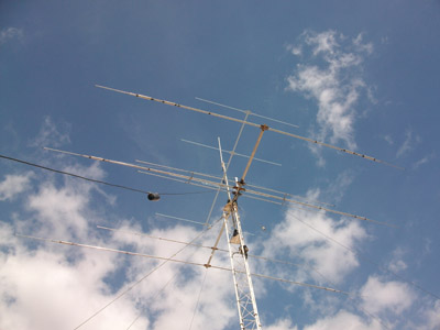
Fig 3.2. Antennas of the EA8DD amateur radio station (courtesy EA8DD).

3.1.2. EA8BPX's log.

In the table 3.3 is a list of the contacts made by the spanish station EA8BPX, placed in the northern area of the Tenerife Island:

Geographic coordinates: 28,45ºN, 16,44ºW.
Geomagnetic coordinates: 33,7ºN, 60,89ºE.
Maidenhead locator: IL18SK.

Date	Hour UTC	Freq (MHz)	Station	RS	City	Country	Locator	Dist (km)	Azimuth (deg)
17/03/2010	22:33	6 m	LU1FVE	55	Castelar	Argentina	FF88XJ	7995	219,2
17/03/2010	22:34	6 m	PP5XX	59	Itapoá	Brazil	GG53QW	6849	212,6
17/03/2010	22:53	6 m	PY0FF	57	Fernando de Noronha	Brazil	HI36TD	3958	207,9
17/03/2010	22:57	6 m	PY2MAJ	54	Sao Paulo	Brazil	GG66RJ	6525	212,2
17/03/2010	23:05	6 m	PY2GH	59	Santo André	Brazil	GG66RI	6529	212,2
18/03/2010	22:49	6 m	PR7AR	55	Paraíba	Brazil	HI23GD	4397	210,4
19/03/2010	21:47	6 m	PT7ZAP	55	Fortaleza	Brazil	HI06RG	4256	217,0
19/03/2010	22:05	6 m	PP1CZ	59	Vitoria/ES	Brazil	GG99UQ	5936	208,0
19/03/2010	22:45	6 m	PU4CQQ	59	Divinopolis	Brazil	GG79NU	6123	212,7
19/03/2010	22:55	6 m	PY2ZXU	57	Santos	Brazil	GG66TB	6549	211,8
20/03/2010	18:39	6 m	LU8EMH	57	Pehuajo	Argentina	FF94BE	8328	216,6
20/03/2010	18:54	6 m	LU8EEM	55	Lincoln	Argentina	FF95GD	8229	216,7
20/03/2010	18:57	6 m	LU5FCI	55	Santo Tomé	Argentina	FF98OI	7933	218,4
20/03/2010	19:14	6 m	9Z4BM	55	San Fernando	Trinidad and Tobago	FK90GG	5079	255,9
20/03/2010	22:27	6 m	PU2CQQ	58	Sao Paulo	Brazil	GG66RK	6521	212,2
20/03/2010	22:27	6 m	PY7XAF	59	Ilha de Itamaracá	Brazil	HI22NE	4465	208,9
24/03/2010	19:17	6 m	KP4EIT	53	Ciales (Puerto Rico)	USA	FK68SI	5207	268,9
24/03/2010	20:08	6 m	TN5SM	55	Desconocida	Congo	JI75PR	4919	131,8
24/03/2010	20:11	6 m	5N7M	59	Abuja	Nigeria	JJ39SB	3293	125,9
25/03/2010	19:52	6 m	PP5XX	59	Itapoá	Brazil	GG53QW	6849	212,6
01/04/2010	17:25	6 m	LU1DMA	59	Buenos Aires	Argentina	GF05PH	8083	215,0
01/04/2010	17:30	6 m	LU6DLB	52	Buenos Aires	Argentina	GF05PH	8083	215,0
01/04/2010	17:34	6 m	LU8EMH	55	Buenos Aires	Argentina	FF94BE	8328	216,3
01/04/2010	17:41	6 m	CX5CR	51	Montevideo	Uruguay	FF82HH	8552	216,0
01/04/2010	17:41	6 m	LW3EX	53	Buenos Aires	Argentina	GF05RL	8062	215,0
01/04/2010	18:31	6 m	LU5CAB	57	Buenos Aires	Argentina	GF05SJ	8065	214,9
01/04/2010	18:32	6 m	LU8ADX	53	Buenos Aires	Argentina	GF05HJ	8108	215,5

Table 3.3. Stations contacted by EA8BPX.

The table 3.4 shows more information about those radio contacts:

LST EA8: local solar time in the Canary Islands.
Lat/Long GEO: geographic coordinates of the stations contacted.
Lat/Long MAG: geomagnetic coordinates of the stations contacted.
LST: local solar time at the location of the station contacted.
LST Diff: difference of local solar time between the stations at both extremes of the radio link.

Date	LST EA8	Station	Locator	Lat GEO	Long GEO	Lat MAG	Long MAG	LST	LST Diff
17/03/2010	21:18	LU1FVE	FF88XJ	-31,60417	-62,04167	-21,76	9,33	18:16	3:02
17/03/2010	21:19	PP5XX	GG53QW	-26,06250	-48,62500	-16,86	22,07	19:11	2:08
17/03/2010	21:38	PY0FF	HI36TD	-3,85417	-32,37500	3,82	39,84	20:35	1:03
17/03/2010	21:42	PY2MAJ	GG66RJ	-23,60417	-46,54167	-14,55	24,22	19:42	2:00
17/03/2010	21:50	PY2GH	GG66RI	-23,64583	-46,54167	-14,59	24,21	19:50	2:00
18/03/2010	21:35	PR7AR	HI23GD	-6,85417	-35,45833	1,17	36,46	20:19	1:16
19/03/2010	20:33	PT7ZAP	HI06RG	-3,72917	-38,54167	4,58	33,72	19:05	1:28
19/03/2010	20:51	PP1CZ	GG99UQ	-20,31250	-40,29167	-11,76	30,44	19:16	1:35
19/03/2010	21:31	PU4CQQ	GG79NU	-20,14583	-44,87500	-11,22	26,08	19:37	1:54
19/03/2010	21:41	PY2ZXU	GG66TB	-23,93750	-46,37500	-14,89	24,35	19:41	2:00
20/03/2010	17:25	LU8EMH	FF94BE	-35,81250	-61,87500	-25,97	9,32	14:24	3:01
20/03/2010	17:40	LU8EEM	FF95GD	-34,85417	-61,45833	-25,03	9,73	14:40	3:00
20/03/2010	17:43	LU5FCI	FF98OI	-31,64583	-60,79167	-21,84	10,47	14:46	2:57
20/03/2010	18:00	9Z4BM	FK90GG	10,27083	-61,45833	20,07	11,28	15:00	3:00
20/03/2010	21:13	PU2CQQ	GG66RK	-23,56250	-46,54167	-14,50	24,22	19:13	2:00
20/03/2010	21:13	PY7XAF	HI22NE	-7,81250	-34,87500	0,15	36,94	20:00	1:13
24/03/2010	18:04	KP4EIT	FK68SI	18,35417	-66,45834	28,29	6,21	14:44	3:20
24/03/2010	18:55	TN5SM	JI75PR	-4,27083	15,29167	-3,77	86,81	21:02	2:07
24/03/2010	18:58	5N7M	JJ39SB	9,06250	7,54167	10,69	81,48	20:34	1:36
25/03/2010	18:40	PP5XX	GG53QW	-26,06250	-48,62500	-16,86	22,07	16:31	2:09
01/04/2010	16:15	LU1DMA	GF05PH	-34,68750	-58,70833	-24,95	12,23	13:26	2:49
01/04/2010	16:20	LU6DLB	GF05PH	-34,68750	-58,70833	-24,95	12,23	13:31	2:49
01/04/2010	16:24	LU8EMH	FF94BE	-35,81250	-61,87500	-25,97	9,32	13:22	3:02
01/04/2010	16:31	CX5CR	FF82HH	-37,68750	-63,37500	-27,81	7,91	13:23	3:08
01/04/2010	16:31	LW3EX	GF05RL	-34,52083	-58,54167	-24,79	12,39	13:42	2:49
01/04/2010	17:21	LU5CAB	GF05SJ	-34,60417	-58,45833	-24,88	12,46	14:33	2:48
01/04/2010	17:22	LU8ADX	GF05HJ	-34,60417	-59,37500	-24,84	11,63	14:30	2:52

Table 3.4. Local solar time and geomagnetic coordinates of the stations contacted by EA8BPX.

3.2. Statistical analysis.

In this section a statistical analysis is applied to the logs, paying attention to three parameters: azimuth and distance from the Canary Islands and hourly distribution.

3.2.1. Azimuth-distance distribution.

The figure 3.3 shows the azimuth-distance distribution of the radio contacts made by EA8DD.

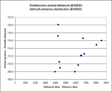
Fig 3.3. Azimuth-distance distribution of the radio contacts from the Canary Islands (EA8DD).

The figure 3.4 shows the azimuth-distance distribution of the radio contacts made by EA8BPX.

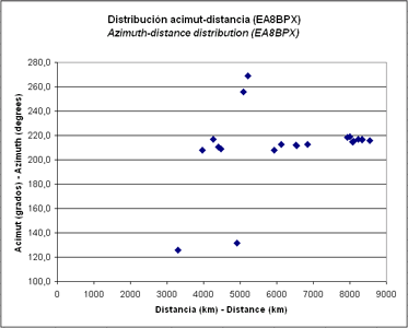
Fig 3.4. Azimuth-distance distribution of the radio contacts from the Canary Islands (EA8BPX).

Finally, the figure 3.5 shows the global azimuth-distance distribution of all the radio contacts, considering both stations.

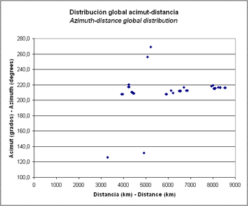
Fig 3.5. Global azimuth-distance distribution of all the radio contacts from the Canary Islands.

We can see 4 big groups, which can be described as follows:

QSO 4200: stations contacted at a distance of around 4200 km, with an azimuth of about 212º, around an intermediate point with geographic coordinates 5,27ºS-35,85ºW and geomagnetic coordinates 2,98ºN-36,57ºE and a local solar time difference of 1:17 with the Canary Islands.
QSO 6400: stations contacted at a distance of around 6400 km, with an azimuth of about 212º, around an intermediate point with geographic coordinates 23,37ºS-46,07ºW and geomagnetic coordinates 14,36ºS-25,41ºE and a local solar time difference of 3:12 with the Canary Islands.
QSO 8200: stations contacted at a distance of around 8200 km, with an azimuth of about 216º, around an intermediate point with geographic coordinates 34,83ºS-60,54ºW and geomagnetic coordinates 25,04ºS-10,57ºE and a local solar time difference of 4:07 with the Canary Islands.
Others: stations contacted not included in any of the previously defined groups.

The groups QSO 4200, QSO 6400 and QSO 8200 are within azimuths of about 212º-216º from the Canary Islands. The stations which belong to the group "Others" are within entirely different azimuths.

3.2.2. Hourly distribution.

The figure 3.6 shows the hourly distribution of all the radio contacts.

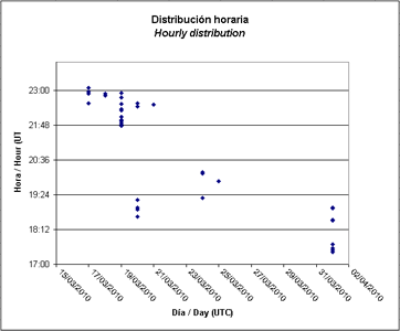
Fig 3.6. Distribución horaria de todos los contactos desde las Islas Canarias.

We can see the time windows shown in the table 3.3.

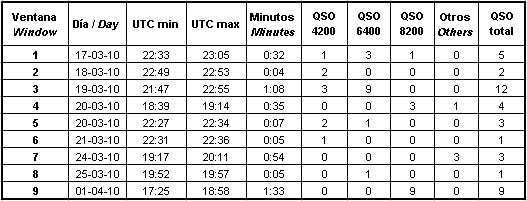
Table 3.3. Time windows of the contacts.

An explanation of each column follows:

Window: ID number for each opening, which will be used from now onwards.
Day: day of the opening.
UTC min/max: time window (UTC) of each opening.
Minutes: duration of each opening (minutes).
QSO 4200: number of QSO with stations included in the group "QSO 4200".
QSO 6400: number of QSO with stations included in the group "QSO 6400".
QSO 8200: number of QSO with stations included in the group "QSO 8200".
Others: number of QSO with stations included in the group "Others".
QSO total: total number of QSO in each window.

We can see that the duration of each aperture was from 5 minutes at minimum to 1 hour and 33 minutes at maximum.

The window 1 took place the day 03/17/2010 between 22:33-23:05 UTC (32 minutes). Stations of the groups QSO 4200, QSO 6400 and QSO 8200 were contacted. It is the only window with contacts of these three groups.

The window 2 took place the day 03/18/2010 between 22:49-22:53 UTC, lasting barely 4 minutes. There were contacts with stations of the group QSO 4200 only.

The window 3 took place the day 03/19/2010 between 21:47-22:55 UTC (1 hour and 8 minutes). It's the window with more contacts, but only with stations of the groups QSO 4200 and QSO 6400.

The window 4 took place the day 03/20/2010 between 18:39-19:14 UTC, lasting 35 minutes. It was the first opening of the two ocurred this day. Oddly, only stations of the group QSO 8200 were contacted, without traces of the other groups nearest to the Canary Islands.

The window 5 took place the same day 03/20/2010 between 22:27-22:34 UTC (7 minutes). There were contacts with stations of the groups QSO 4200 and QSO 4600.

The window 6 took place the day 03/21/2010 between 22:31-22:36 UTC, lasting barely 5 minutes and with only one contact with a station of the group QSO 4200.

The window 7 took place 3 days later, on the 03/24/2010, between 19:17-20:11 UTC (54 minutes). During this window, there weren't contacts with stations of the three big groups, but with Puerto Rico, Congo and Nigeria instead, placed at azimuths absolutely different of the main one.

The window 8 took place the day 03/25/2010, between 19:52-19:57 UTC, lasting 5 minutes only, with only one contact with a station of the group QSO 6400.

And finally, the window 9 took place several days later, on the 04/01/2010, between 17:25-18:58 UTC, being the longest opening with 1 hour and 33 minutes. There were 9 contacts, all of them with stations of the group QSO 8200. As in the window 4, there weren't traces of the other groups nearest to the Canary Islands

Please note that the vernal equinox occured on 20/03/2010 at 16:31 UTC.

3.3. Methodology used in the calculations.

Currently there is no available technical data about the equipment used by the stations in Brazil, so we will assume that they used identical antenna gain, RF power and receiver sensitivity to the used by the EA8DD station.

The analysis will take into account several aspects such as the geometry of the links, the power budgets and the computation of the maximum usable frequency from critical frequency values measured by ionosondes.

In the case of the simple propagation modes, the geometrical calculations are based on trigonometry, using the approach of straight rays not affected by refraction nor scattering [Ref.Pellejero].

The power budget calculations are based on the computation of free spaces losses determined by the transmission equation, making also the following theoretical approaches about the ionospheric propagation losses [Ref.Pellejero]:

First reflection in the ionosphere: 5 dB.
Second reflection in the ionosphere: 5 dB.
Third reflection in the ionosphere: 3,5 dB.
Each one of the other reflections in the ionosphere: 2,5 dB.
Each one of the reflections on the Earth's surface: 3,5 dB.

Finally, in some cases the maximum usable frequency of the different layers of the ionosphere is extrapolated from the critical frequency values measured by ionosondes, following the method also described in [Ref.Pellejero].

4. Analysis of the ionospheric conditions.

We have gathered scientific data from several ionospheric sounding stations around the Equator, with the goal of analyzing the ionization levels in the different layers of the ionosphere, during the days and hours of the contacts. I have collected data from the stations indicated in the table 4.1, being necessary to emphasize that in some cases the distance between the sounding station and the radio path is quite high and this fact could detract from the validity of the data for the propagation analysis of the radio links under study. In spite of this fact, those data can be valuable to get an idea of the general conditions of ionization in similar latitudes.

Ionosonde	Country	URSI code	Latitude	Longitude
Tucumán	Argentina	TUJ2O	26,9ºS	65,4ºW
Fortaleza	Brazil	FZA0M	3,8ºS	38ºW
Sao Luis	Brazil	SAA0K	2,6ºS	44,2ºW
Cachoeira Paulista	Brazil	CAJ2M	23,20ºS	45,8ºW
Isla Ascensión	UK	AS00Q	7,95ºS	14,4ºW
Kwajalein	Marshall Islands	KJ609	9ºN	167,2ºE

Table 4.1. Ionospheric sounding stations checked

The ionospheric sounding stations checked make vertical soundings every 10 or 15 minutes in order to measure several parameters of the ionosphere, such as the presence of the different layers, their critical frequencies or they thickness.

As we may expect, only the first samples of each day (until 20:40 UTC maximum) show the presence of the E layer.

We have also collected data about total electron content (TEC) measurements and ionospheric scintillation maps, provided to the public by several agencies devoted to the study of space weather.

4.1. Space weather conditions.

The table 4.2 shows the most significative space weather parameters during the days of the contacts (source: Joint USAF/NOAA Solar and Geophysical Activity Summary).

Day	SFI	SSN	Ap	Kp max	Geomag. Act.
03/17/2010	87	28	7	4	Quiet
03/18/2010	86	27	5	3	Quiet
03/19/2010	84	24	4	2	Quiet
03/20/2010	84	25	7	3	Quiet
03/21/2010	85	25	2	1	Quiet
03/24/2010	84	27	3	2	Quiet
03/25/2010	88	25	5	2	Quiet
04/01/2010	79	25	12	4	(*)

Tabla 4.2. Space weather conditions during the days of the contacts

(*) The geomagnetic field has been predominantly at unsettled levels with an isolated period of major storming at high lattitudes (12:00-15:00Z).

An explanation of each parameter follows:

SFI: Solar Flux Index in the 10,7 cm band.
SSN: Sunspot Number.
Ap, Kp: planetary geomagnetic activity indices.
Geomag. Act: remarks about the geomagnetic activity.

The conditions are typical of day of the minimum of the solar cycle, without relevant geomagnetic activity.

4.2. Contenido total de electrones (TEC).

The figure 4.1 shows a capture of the total electron content (TEC) provided by the Space Weather Prediction Center (SWPC) of the north-american agency NOAA, corresponding to the 22:50 UTC hours of 03/18/2010. A line has been superimposed, showing the trajectory of the radio links under study.

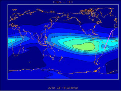
Fig 4.1. TEC registered by NOAA (United States).

There is no available data for the other dates. In the figure, in the area of the radio path, the equatorial anomaly is clear: TEC both sides of the Equator is higher than in the Equator itself.

4.3. Ionograms.

Ionograms are the graphic result of the measurements made by ionospheric sounding stations, also known as ionosondes, which made steady soundings of the ionosphere by means of transmitting radio waves at different frequencies, following perpendicular or oblique paths from the Earth's surface. The detection of the reflected waves and the measurement of their travelling time allow to calculate several parameters of the ionosphere, such as the presence of its different layers, their thickness and the critical or cut frequency of each layer.

The ionosondes are also able to detect ionospheric irregularities, which show as range spread (spread-F) in the ionograms [Ref.Reinisch].

We have gathered data from the ionosondes at Tucumán (Argentina), Ascension Island (UK), Fortaleza (Brazil) and Sao Luis (Brazil), being those of interest due to their proximity to the radio paths under study (fig.4.2). We have also checked data from other ionosondes near the Equator, such as Kwajalein (Marshall Islands).

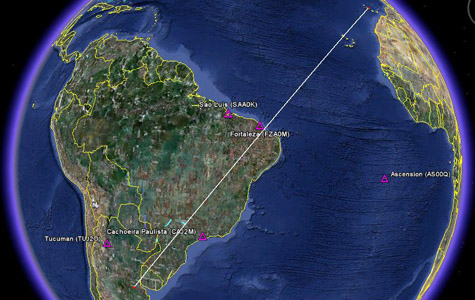
Fig 4.2. Ionospheric sounding stations closest to the radio path.

For each case, we have collected the data in the interval 03/17/2010-03/22/2010, between 20:00 UTC and 23:45 UTC, analyzing the following parameters:

Evolution of the measurements of the critical frequencies of the E layer (foE), the sporadic E layer (foEs) and the F2 layer (foF2) of the ionosphere (vertical incidence).
Evolution of the measurements of the minimum height of the E layer (h'E), the sporadic E layer (h'Es) and the F2 layer (h'F2) of the ionosphere.

Evolution of the predictions of MUF(3000)F2 to try to extrapolate possible cases of MUF(F2) > 50 MHz between the Canary Islands and Brazil. The MUF(3000)F2 is a theoretical extrapolation of the MUF for paths of 3000 km in length from the ionosonde, predicted from the foF2 and other parameters.

Occurrences of range spread to see possible ionospheric irregularities supposedly able to grant duct propagation (TEP).

In order to try to identify characteristic patterns of those parameters during the days of the contacts, a wider time margin has been analyzed also, between 03/05/2010-04/05/2010.

Knowing the critical frequency of each layer of the ionosphere (fo), given as a measured value by the ionosonde, we
can determine the maximum usable frequency (MUF) for oblique incidence using the secant law [Ref.Pellejero].

The fig.4.3 shows the minimum fo necessary at a particular altitude to allow a MUF of 50 MHz, working with the antennas pointing to the horizon and using the hyphotesis of straight rays.

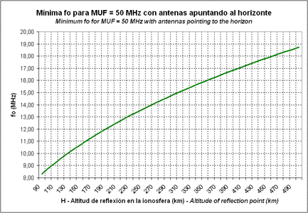
Fig 4.3. Minimum fo required in each layer to allow oblique reflection with MUF = 50 MHz.

In order to allow oblique reflections at 50 MHz in the E layer, the sporadic E layer or the F2 layer, the critical frequencies
measured by the ionosonde must be:

foE > 8,76 MHz (HE = 100 km).
foEs > 8,76 MHz (HEs = 100 km).
foF2 > 25,22 (HF2 = 300 km).

We must consider that those values are related to pure ionospheric reflection. It is common that, before reaching the reflection condition, radio waves are refracted and as a result the rays are bent. This occurs at frequencies even lower than those listed.

4.3.1. Tucumán ionosonde.

This section shows the data collected by the ionospheric sounding station located at Tucumán, Argentina (URSI code TUJ2O), coordinates 26,9ºS / 65,4ºW. The measurements were done between the days 17 and 22 march 2010, in the time window between 20:00 UTC and 23:45 UTC.

In the tables, the empty cells show sounding failures or the absence of data. The values in red match the dates and hours of the radio contacts.

The table 4.3 shows the critical frequency of the F2 layer (foF2) values, measured at Tucumán.

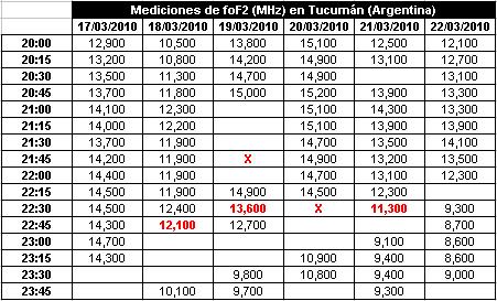
Table 4.3. Measurements of foF2 at Tucumán (Argentina).

Those measurements are plotted in the figure 4.4.

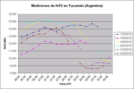
Fig 4.4. Plot of the foF2 values registered at Tucumán (Argentina).

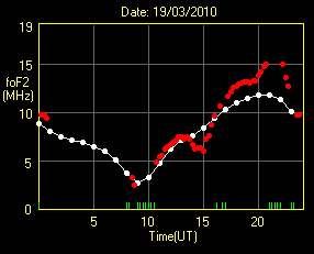
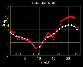
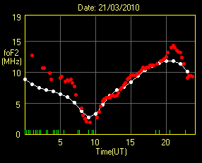
In the figure 4.5, for each indicated date, the red dotted line show the foF2 values measured by the ionosonde and the white dotted line show the foF2 monthly mean expected value.

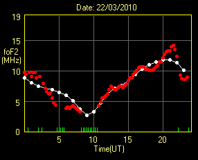Fig 4.5. foF2 deviation from the monthly mean in Tucumán (Argentina).

We can see that during the days of the radio contacts, from 17-20 hours UTC to more than 23 hours UTC, the foF2 values were up to 3 MHz higher that the monthly mean. That is, there were exceptional ionization conditions.

The table 4.4 shows the prediction of the MUF for a range of 3000 km, using reflection at the F2 layer, known as MUF(3000)F2, from the Tucumán station for the same time intervals.

Table 4.4. MUF(3000)F2 predicted at Tucumán (Argentina).

The prediction is plotted in the figure 4.6.

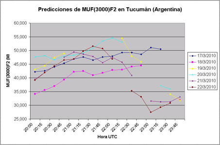
Fig 4.6. Plot of the MUF(3000)F2 prediction at Tucumán (Argentina).

It can be seen that MUF(3000)F2 was over 50 MHz for several hours, the days 17, 19, 20 and 22.

It is necessary to take into account that in the ionograms offered by this station, it is difficult to characterize range spread conditions, which for sure took place as shown by other nearby ionosondes. During range spread episodes, the measurements of the ionosonde may have siginificative errors.

4.3.2. Ascension Island ionosonde.

This section shows the data collected by the ionospheric sounding station located at Ascension Island, UK (URSI code AS00Q), coordinates 7,95ºS / 14,4ºW. The measurements were done between the days 17 and 22 march 2010, in the time window between 20:00 UTC and 23:45 UTC.

The figure 4.7 shows the plot of the measurements of the cut frequencies corresponding to the F2 layer (foF2, red plot), the E layer (foE, blue plot) and the sporadic E layer (foEs, yellow plot).

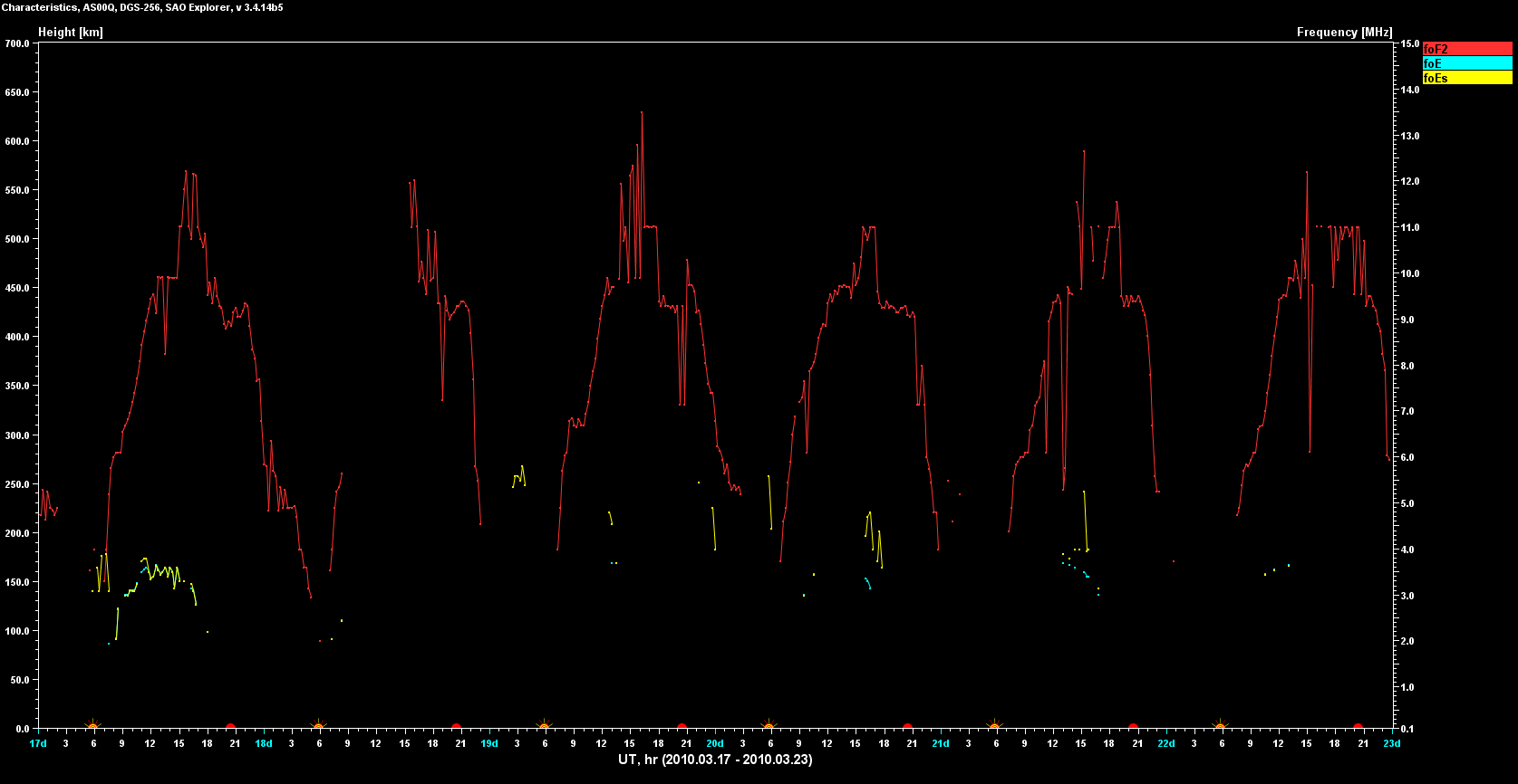
Fig 4.7. Plot of the foF2, foE and foEs values registered at Ascension Island (UK).
Click on the image to see a larger version

The figure 4.8 shows the plot of the measurements of the minimum altitudes corresponding to the F2 layer (h'F2, red plot), the E layer (h'E, blue plot) and the sporadic E layer (h'Es, yellow plot).

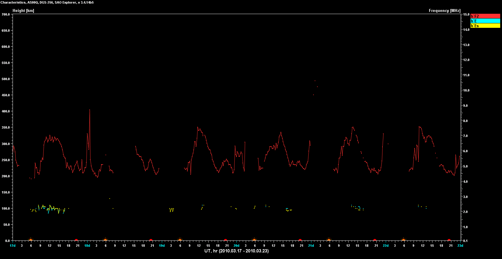
Fig 4.8. Plot of the h'F2, h'E and h'Es values registered at Ascension Island (UK).
Click on the image to see a larger version

The figure 4.9 shows the plot of the measurements of range spread in the F layer (QF, pink plot) and in the E layer (QE, blue plot).

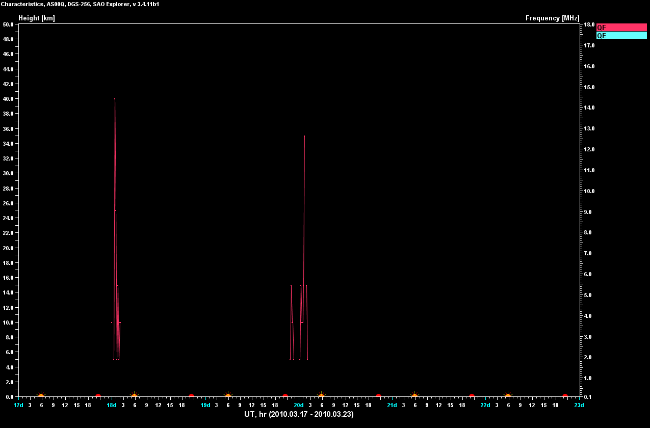
Fig.4.9. Plot of the QF and QE values registered at Ascension Island (UK).
Click on the image to see a larger version

The figure 4.10 shows an example of range spread, corresponding to the day 03/19/2010 at 22:30 UTC, the hour of one of the radio contacts.

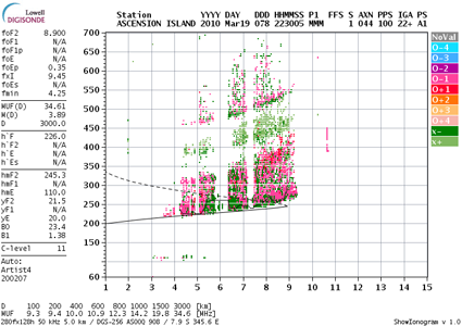
Fig 4.10. Range spread or spread-F observed at Ascension Island.

The figure 4.11 shows the prediction of the MUF for a range of 3000 km, using reflection at the F2 layer, known as MUF(3000)F2, from the Ascension Island station for the same time intervals.

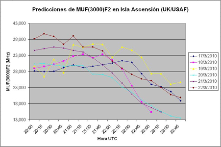
Fig 4.11. Plot of the MUF(3000)F2 prediction at Ascension Island.

It can be seen that MUF(3000)F2 was always below 39 MHz. Both foF2 and MUF(3000)F2 plots follow a descending trend with time, due to the effects of electron recombination in the ionosfere at dusk. The effects of range spread seem not to affect much to the measurements and the predictions.

4.3.3. Fortaleza ionosonde.

This section shows the data collected by the ionospheric sounding station located at Fortaleza, Brazil (URSI code FZA0M), coordinates 3,8ºS / 38ºW. There isn't available data from the day 17.

The figure 4.12 shows the plot of the measurements of the cut frequencies corresponding to the F2 layer (foF2, red plot), the E layer (foE, blue plot) and the sporadic E layer (foEs, yellow plot), registered at Fortaleza between the days 03/05/2010 and 04/06/2010.

Fig 4.12. Plot of the foF2, foE and foEs values registered at Fortaleza (Brazil) - General.
Click on the image to see a larger version

The figure 4.13 is a detail of those measurements between the days 03/17/2010 and 03/22/2010.

Fig 4.13. Plot of the foF2, foE and foEs values registered at Fortaleza (Brazil) - Detail.
Click on the image to see a larger version

We can see that during the time intervals where the contacts were established, the Es layer was not present. However, we may stress that this layer could be hidden in the ionograms during the range spread espisodes.

The figure 4.14 shows the plot of the measurements of the minimum altitudes corresponding to the F2 layer (h'F2, red plot), the E layer (h'E, blue plot) and the sporadic E layer (h'Es, yellow plot), registered at Fortaleza between the days 03/05/2010 and 04/06/2010.

Fig 4.14. Plot of the h'F2, h'E and h'ES values registered at Fortaleza (Brazil) - General.
Click on the image to see a larger version

The figure 4.15 is a detail of those measurements between the days 03/17/2010 and 03/22/2010.

Fig 4.15. Plot of the h'F2, h'E and h'ES values registered at Fortaleza (Brazil) - Detail.
Click on the image to see a larger version

The figure 4.16 shows the plot of the measurements of range spread in the F layer (QF, pink plot) and in the E layer (QE, blue plot).

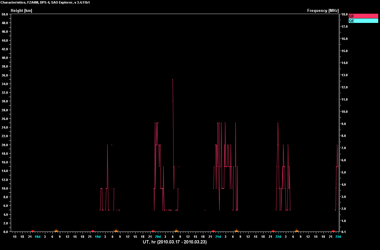
Fig.4.16. Plot of the QF and QE values registered at Fortaleza (Brasil) .
Click on the image to see a larger version

The figure 4.17 shows an example of range spread, corresponding to the day 03/19/2010 at 22:30 UTC, the hour of one of the radio contacts.

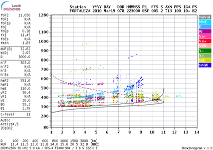
Fig 4.17. Range spread or spread-F observed at Fortaleza (Brazil).

The figure 4.18 shows the plot of the MUF(3000)F2 prediction at Fortaleza between the days 03/05/2010 and 04/06/2010.

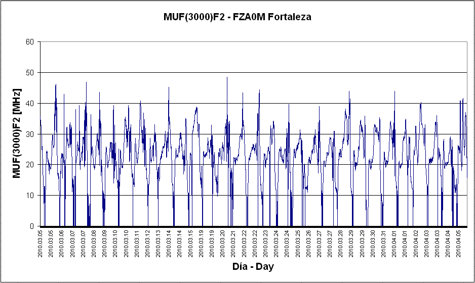
Fig 4.18. MUF(3000)F2 predicted at Fortaleza (Brasil) - General.
Click on the image to see a larger version

The figure 4.19 shows a detail of this prediction between the days 03/17/2010 and 03/22/2010.

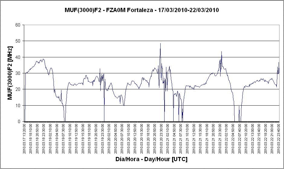
Fig 4.19. MUF(3000)F2 predicted at Fortaleza (Brazil) - Detail.
Click on the image to see a larger version

To summarize, the table 4.5 shows the maximum values of all the parameters analysed during the time windows of the radio contacts (table 3.3).

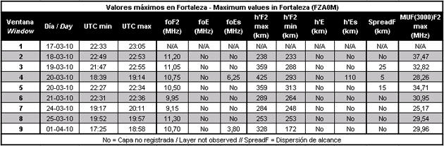
Table 4.5. Values of interest at Fortaleza (Brazil) during the time windows of the contacts

It can be seen that MUF(3000)F2 was below 38 MHz during all the windows. We can see also some differences between the data from this ionosonde (latitude 3,8ºS) and those from the ionosonde in the Ascension Island (7,95ºS):

In absence of range spread, the foF2 values are slightly higher in Fortaleza.
During range spread conditions, the measurements at Fortaleza seem to be more affected, presenting great variations probably due to autoscaling errors.
We cannot see a descending trend in the foF2 and MUF(3000)F2 plots, a fact most probably related to the mentioned autoscaling errors.
The range spread is observed about 30 minutes later in Fortaleza. One possible explanation is that the ionospheric irregularities observed at Ascension Island spent this time to be aligned with the geomagnetic field and travel northwest, following a path perpendicular to the magnetic Equator. Other possibility could be that there were different irregularities.

4.3.4. Sao Luis ionosonde.

This section shows the data collected by the ionospheric sounding station located at Sao Luis, Brazil (URSI code SAA0K), coordinates 2,6ºS / 44,2ºW.

The figure 4.20 shows the plot of the measurements of the cut frequencies corresponding to the F2 layer (foF2, red plot), the E layer (foE, blue plot) and the sporadic E layer (foEs, yellow plot), registered at Sao Luis between the days 03/05/2010 and 04/06/2010.

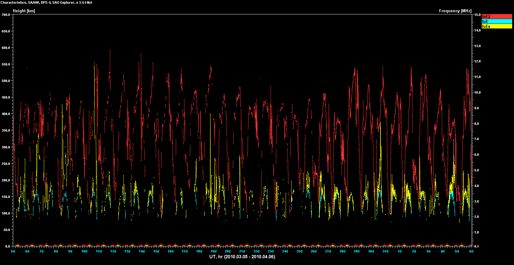
Fig 4.20. Plot of the foF2, foE and foEs values registered at Sao Luis (Brazil) - General.
Click on the image to see a larger version

The figure 4.21 is a detail of those measurements between the days 03/17/2010 and 03/22/2010.

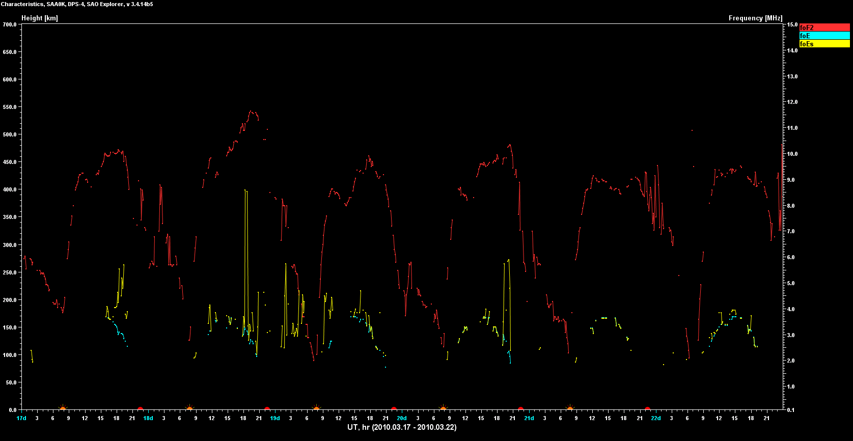
Fig 4.21. Plot of the foF2, foE and foEs values registered at Sao Luis (Brazil) - Detail.
Click on the image to see a larger version

The figure 4.22 shows the plot of the measurements of the minimum altitudes corresponding to the F2 layer (h'F2, red plot), the E layer (h'E, blue plot) and the sporadic E layer (h'Es, yellow plot), registered at Fortaleza between the days 03/05/2010 and 04/06/2010.

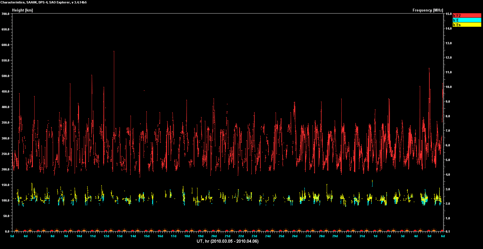
Fig 4.22. Plot of the h'F2, h'E and h'Es values registered at Sao Luis (Brazil) - General.
Click on the image to see a larger version

The figure 4.23 is a detail of those measurements between the days 03/17/2010 and 03/22/2010.

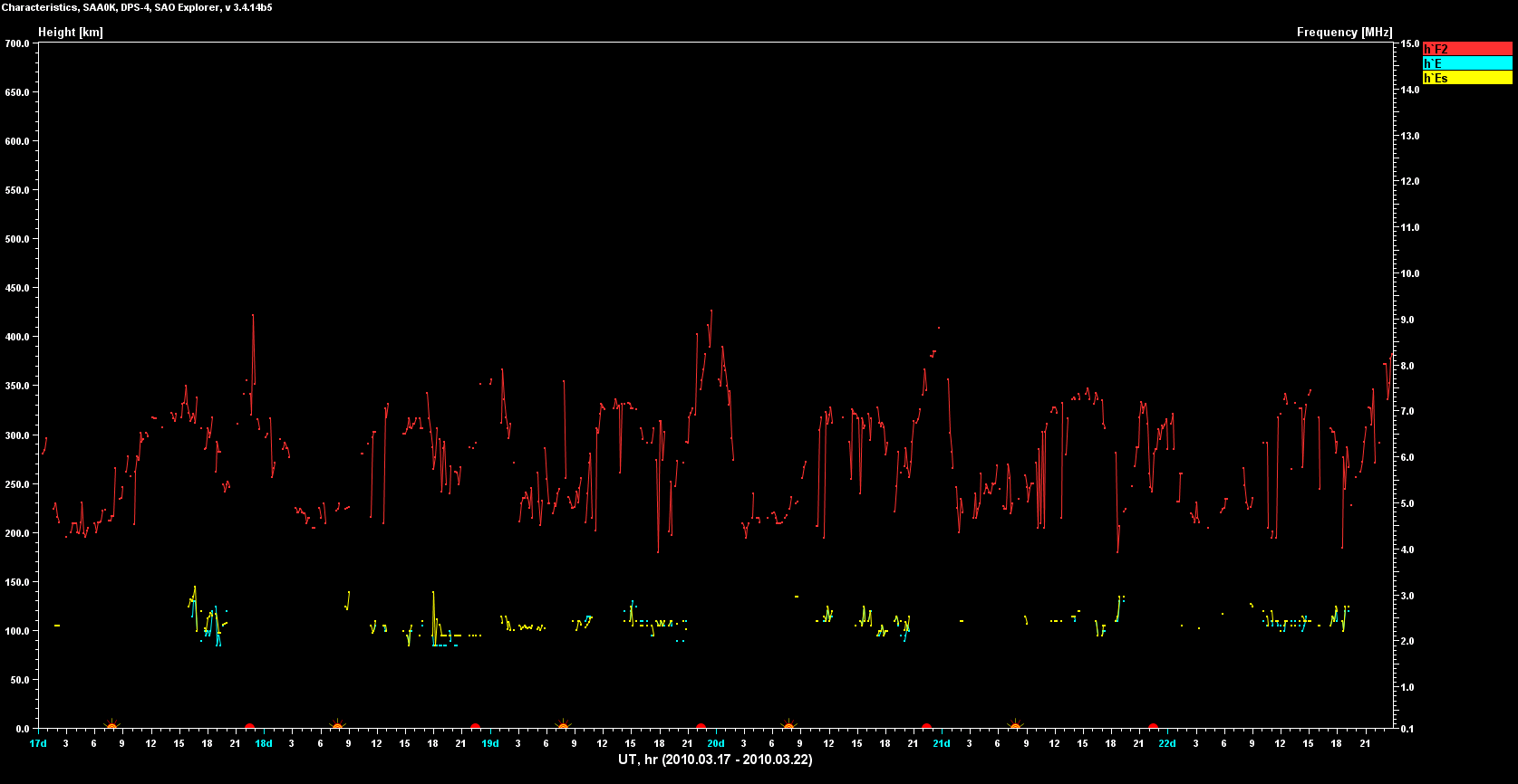
Fig 4.23. Plot of the h'F2, h'E and h'Es values registered at Sao Luis (Brazil) - Detail.
Click on the image to see a larger version

We can see the presence of the sporadic layer Es during almost all the hours of the time interval under study for the day 18th and only at the beginning of the interval the days 19th and 20th. It is necessary to take into account that the ionosonde detected spread-F during this interval the days 19th and 20th, so those measurements could be subject to errors. The maximum foEs observed is 5,850 MHz, indicating high levels of ionization but seemingly not enough to reflect radio waves of 50 MHz with oblique incidence. The Es layer was present during only one of the contacts, the day 18th at 22:50 UTC.

The figure 4.24 shows the plot of the measurements of range spread in the F layer (QF, pink plot) and in the E layer (QE, blue plot).

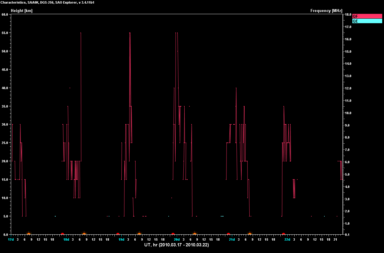
Fig.4.24. Plot of the QF and QE values registered at Sao Luis (Brasil) .
Click on the image to see a larger version

The figure 4.25 shows an example of range spread, corresponding to the day 03/19/2010 at 22:30 UTC, the hour of one of the radio contacts.

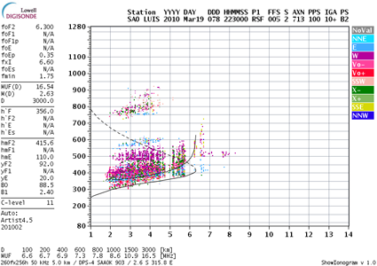
Fig 4.25. Range spread or spread-F observed at Sao Luis (Brazil).

In this case, we can see that range spread took place during the most time of all the analyzed cases. Every day from 22:00 UTC the foF2 measurements suffer from high variations, most probably due to autoscaling errors as a consequence of range spread.

The figure 4.26 shows the prediction of the MUF for a range of 3000 km, using reflection at the F2 layer, known as MUF(3000)F2, from the Sao Luis station for the same time intervals.

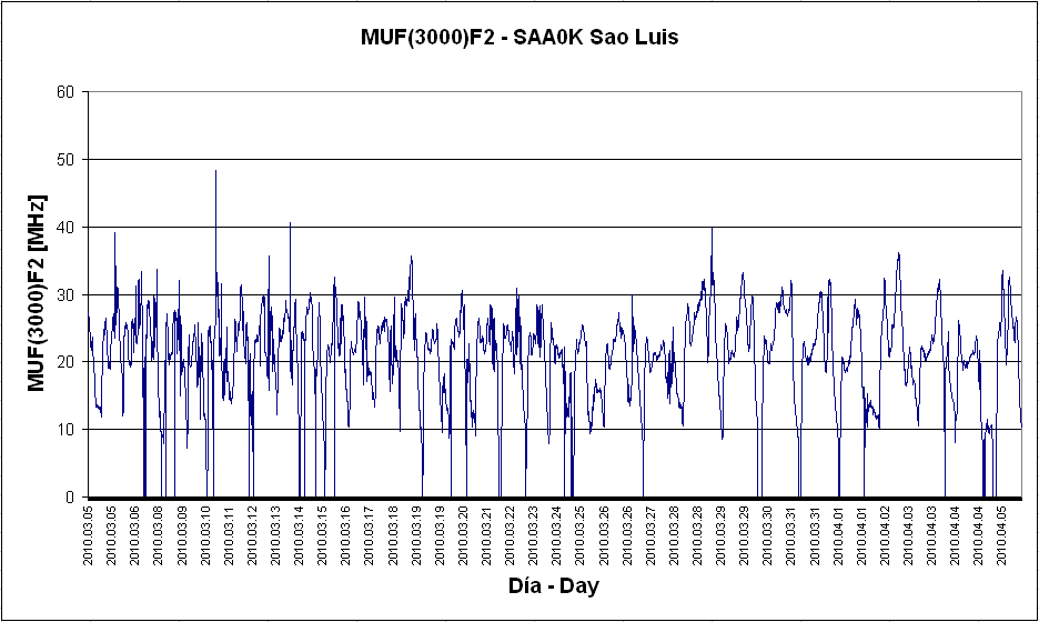
Fig 4.26. MUF(3000)F2 predicted at Sao Luis (Brazil) - General.
Click on the image to see a larger version

The figure 4.27 shows a detail of this prediction between the days 03/17/2010 and 03/22/2010.

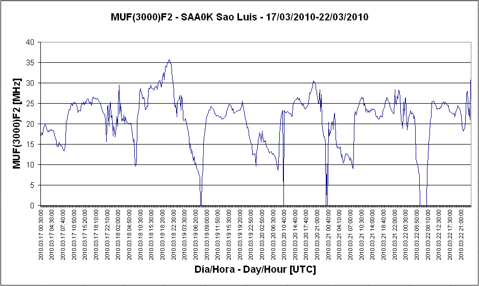
Fig 4.27. MUF(3000)F2 predicted at Sao Luis (Brazil) - Detail.
Click on the image to see a larger version

To summarize, the table 4.6 shows the maximum values of all the parameters analysed during the time windows of the radio contacts (table 3.3).

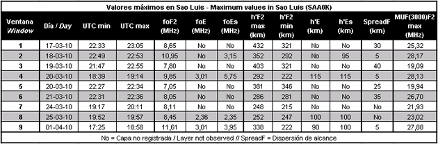
Table 4.6. Values of interest at Sao Luis (Brazil) during the time windows of the contacts

The MUF(3000)F2 predicted was always below 29 MHz during all the openings.

4.3.5. Cachoeira Paulista ionosonde.

This section shows the data collected by the ionospheric sounding station located at Cachoeira Paulista, Brazil (URSI code CAJ2M), coordinates 23,20ºS / 45,8ºW.

The figure 4.28 shows the plot of the measurements of the cut frequencies corresponding to the F2 layer (foF2, red plot), the E layer (foE, blue plot) and the sporadic E layer (foEs, yellow plot), registered at Cachoeira Paulista between the days 03/05/2010 and 04/06/2010.

Fig 4.28. Plot of the foF2, foE and foEs values registered at Cachoeira Paulista (Brazil) - General.
Click on the image to see a larger version

The figure 4.29 is a detail of those measurements between the days 03/17/2010 and 03/22/2010.

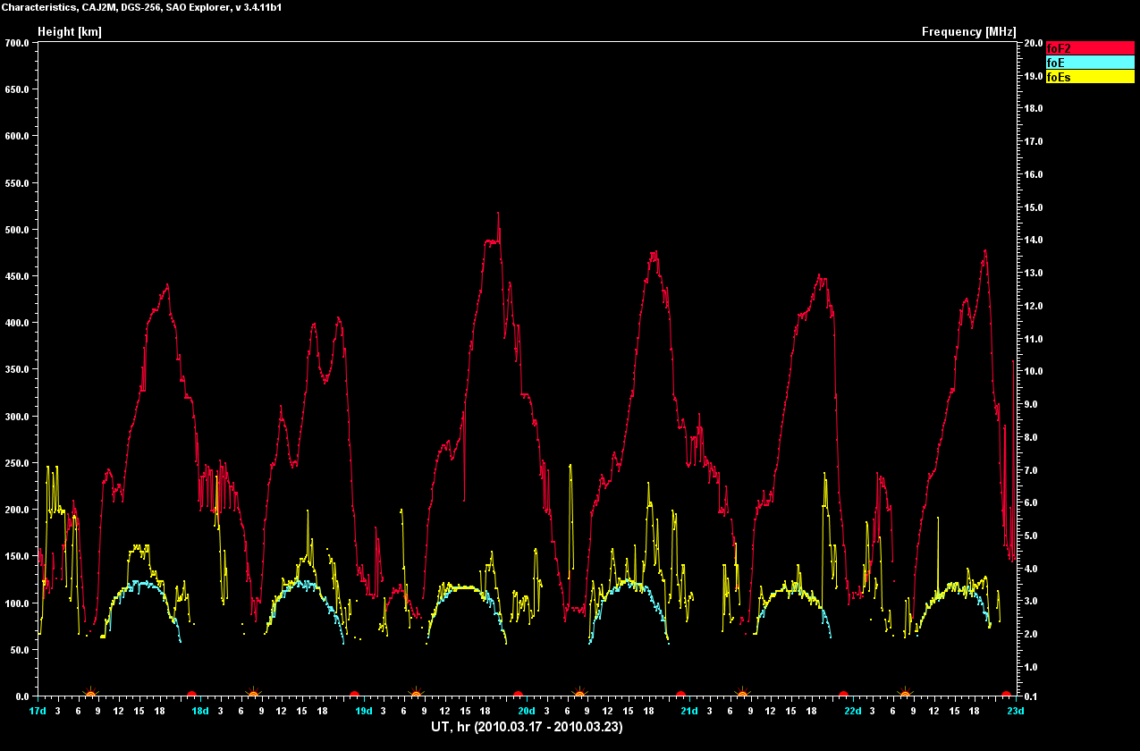
Fig 4.29. Plot of the foF2, foE and foEs values registered at Cachoeira Paulista (Brazil) - Detail.
Click on the image to see a larger version

The figure 4.30 shows the plot of the measurements of the minimum altitudes corresponding to the F2 layer (h'F2, red plot), the E layer (h'E, blue plot) and the sporadic E layer (h'Es, yellow plot), registered at Cachoeira Paulista between the days 03/05/2010 and 04/06/2010.

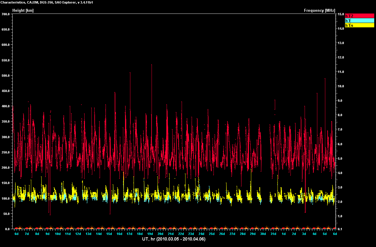
Fig 4.30. Plot of the h'F2, h'E and h'Es values registered at Cachoeira Paulista (Brazil) - General.
Click on the image to see a larger version

The figure 4.31 is a detail of those measurements between the days 03/17/2010 and 03/22/2010.

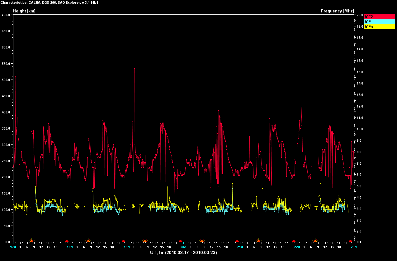
Fig 4.31. Plot of the h'F2, h'E and h'Es values registered at Cachoeira Paulista (Brazil) - Detail.
Click on the image to see a larger version

The figure 4.32 shows the plot of the measurements of range spread in the F layer (QF, pink plot) and in the E layer (QE, blue plot).

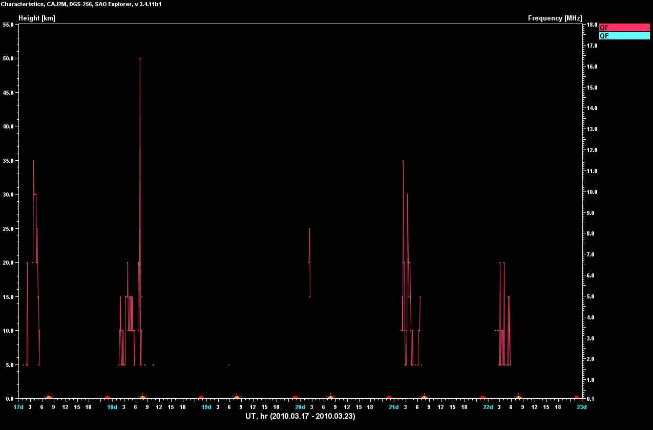
Fig.4.32. Plot of the QF and QE values registered at Cachoeira Paulista (Brasil) .
Click on the image to see a larger version

We can see that there wasn't any range spread event during the hours of the contacts in the examined window.

The figure 4.33 shows the plot of the MUF(3000)F2 prediction between the days 03/05/2010 and 04/06/2010.

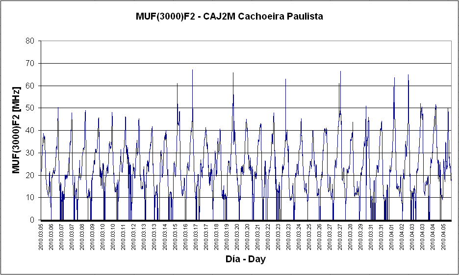
Fig 4.33. MUF(3000)F2 predicted at Cachoeira Paulista (Brasil) - General.
Click on the image to see a larger version

The figure 4.34 shows a detail of this prediction between the days 03/17/2010 and 03/22/2010.

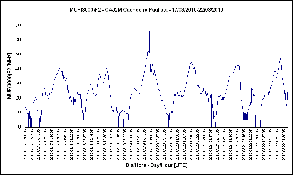
Fig 4.34. MUF(3000)F2 predicted at Cachoeira Paulista (Brasil) - Detail.
Click on the image to see a larger version

To summarize, the table 4.7 shows the maximum values of all the parameters analysed during the time windows of the radio contacts (table 3.3).

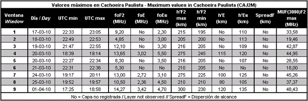
Table 4.7. Values of interest at Cachoeira Paulista (Brazil) during the time windows of the contacts

The MUF(3000)F2 predicted was always below 49 MHz during all the openings.

4.4. Ionospheric scintillation maps.

The European Space Agency (ESA) manages the Ionospheric Scintillations Monitoring Service, as a part of its Space Weather European Network (SWENET).

Scintillation is the phenomenon suffered by radio waves travelling through regions of the ionosphere affected by irregularities which deplete about 10% the density of ionization, causing diffraction and scattering. This may affect the satellite communication systems and due to this is steadily monitored, employing terrestrial networks such as the based on the analysis of the GPS constellation signals.

At every hour the radio contacts where made (see table 3.3), in the Cape Verde Islans area the ESA network detected high levels of scintillation (red spots in the map). This could be a good indicator of the existence of ionospheric irregularities in the area, such as the described in section 2.2.

The figure 4.35 shows the scintillation map of 03/18/2010 at 22:00 UTC.

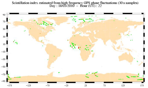
Fig 4.35. Scintillation map for the day 03/18/2010 22:00 UTC (ESA/SWENET).

The figure 4.36 shows the scintillation map of 03/19/2010 at 22:00 UTC.

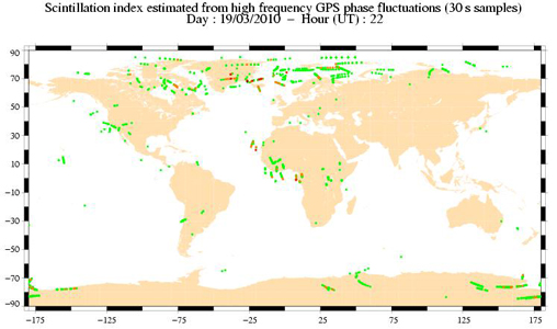
Fig 4.36. Scintillation map for the day 03/19/2010 22:00 UTC (ESA/SWENET).

The figure 4.37 shows the scintillation map of 03/20/2010 at 22:00 UTC.

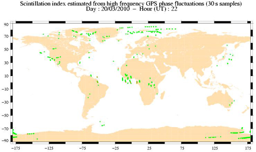
Fig 4.37. Scintillation map for the day 03/20/2010 22:00 UTC (ESA/SWENET).

The figure 4.38 shows the scintillation map of 03/21/2010 at 22:00 UTC.

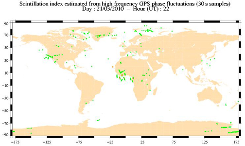
Fig 4.38. Scintillation map for the day 03/21/2010 22:00 UTC (ESA/SWENET).

5. Propagation modes hyphotesis.

From the data analyzed, we can have some conclusions about the ionization levels existing in the area, which may provide an idea of the theoretical MUF between the Canary Islands and Brazil using one or two hops in the F2 layer (1F and 2F modes).

Other possibility is based on the use of the E layer or the sporadic Es layer, through one hop (1E and 1Es modes) or several hops (nE and nEs modes).

Complex modes could also have occurred, combining hops in the F and E layers, such as 1F1E or 1E1F modes.

Finally, some other typical transequatorial modes may have occurred, such as chordal modes in the F layer (FF mode) or duct conduction due to equatorial plasma bubbles (EPB) or a path between the E and F layers.

Determining which propagation mode made this contacts possible is extremelly difficult, mostly if we don't have data about the propagation delay, which could be very helpful to calculate the possible radio paths. In this section we offer different hyphotesis based on the available data.

5.1. One-hop hyphotesis.

This hyphotesis is based on the possibility of the radio link established using only one hop in one of the layers of the ionosphere, by means of reflection or scattering.

M.Dolukhanov devotes a section of his book "Propagation of Radio Waves" [Ref.Dolukhanov] to the propagation of metric waves through scatter from the ionosphere, mode discovered by Baily in 1951. According to Dolukhanov, scattering may take place in the D layer or in the lower part of the E layer at night, providing radio ranges up to 2000 km.

5.1.1. Geometric analysis using straight rays.

In order to check whether this mode of propagation was possible using only one hop through the E layer (E mode) or through a possible sporadic Es layer (Es mode), we can use the geometrical analysis shown in the figure 5.1.

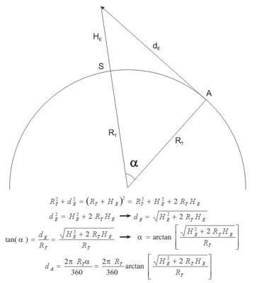
Fig 5.1. Geometry of the link using only one hop.

A = Location of the transmitter at Tenerife (Canary Islands).

S = Projection of the reflection/scattering point in the ionosphere over the Earth's surface.

dE = Distance from the transmitter to the reflection/scattering point in the ionosphere.

HE = Altitude of the reflection/scattering point.

RT = Earth's radius = 6370 km

dA = Arc length between points A and S.

The other half of the radio link would be completely simmetrical to the one shown in the figure.

If we take into account that the transmitter's antenna is pointing to the horizon, following the tangent to the Earth's surface, and that the altitude where reflection/scattering occurs in the E layer is HE = 150 km, we can conclude that this reflection/scattering would have taken place at a point located about 200 km north of the Cape Verde archipelago, whose coordinates are 17,25ºN, 23,52ºW, as shown in the figure 5.2.

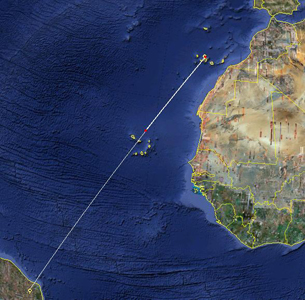
Fig 5.2. Theoretical reflection point at an altitude of 150 km.

This point is 1370 km away from Tenerife (Canary Islands) and 3166 km away from Paraíba (Brazil). Direct reflection or scattering towards Paraíba would be impossible because the path would be under the terrestrial tangent at Paraíba, that is, hidden by the Earth's curvature, excluding extraordinary cases of tropospheric refraction. So there is a very low probability for the E or Es mode to occur between both points.

Following the calculations shown in the figure 5.1, we can determine from which altitude the reflected/scattered ray would reach Paraíba thanks to line of sight conditions, being HE = 425 km, that is, a possible F mode. The reflection/scattering would take place just in the middle point of the path between Tenerife and Paraíba, a point over the Atlantic with coordinates 9,73ºN, 27,16ºW (fig.5.3). The F mode of propagation of radio waves up to 50 MHz has been described by several authors [Ref.Morgan], indicating that diurnal peaks of ionization, low latitude points of reflection and years of maximum sunspot activity are most favorable for such transmission.

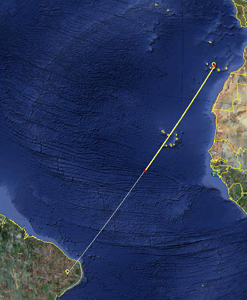
Fig 5.3. Theoretical reflection point at an altitude of 425 km.

5.1.2. Analysis using BeamFinder.

It seems more logical that a reflection in the F layer takes place at an altitude of about HE = 300 km. Considering this geometry, the area where the contacted stations are placed would be out of the expected coverage area for one hop, as shown in the map of the figure 5.4, made with the BeamFinder software [Ref.BeamFinder].

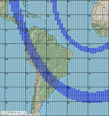
Fig 5.4. Coverage areas in the 1F and 2F modes (courtesy Volker Grassmann, DF5AI).

5.1.3. Ionospheric parabolic model.

In 1990, a study [Ref.Rappaport] tried to justify that some radio links of the Amateur Radio Service in the 50 MHz band with great circle distances between 4.200-6.500 km and up to 10.000 km may have been due to propagation using one or two hops in the F2 layer of the ionosphere, describing the possible geometries with the ionospheric parabolic model. In the fig.5 the results are shown for a maximum free electron density of 3E+12 and different values of the parabolic semi-thickness (150 km, 200 km and 250 km).

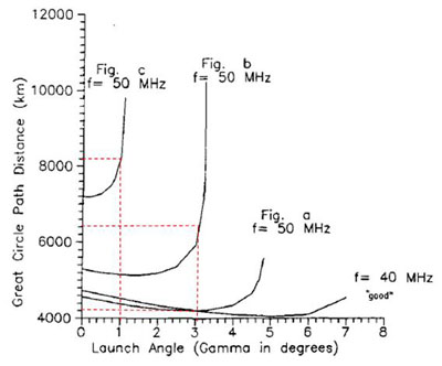
Fig 5.x. Great circle path distances in 50 MHz as a function of the takeoff angle
(Rappaport et Al. model).

Each plot corresponds to a different solution reached using numeric models. The vertical axis is the great circle path distance and the horizontal axis is the antenna's takeoff angle. For the specific parameters evaluated, we can see that using takeoff angles between 1º and 3º, distances corresponding to our groups QSO 4200, QSO 6400 and QSO 8200 are possible. However, it is necessary to remark the lack of data from ionosondes in the estimated ionospheric reflection areas, which would allow to extrapolate the data from the graphs to our study.

5.1.4. Scattering from regular ionization areas.

Another possibility of propagation related to the F layer is the scattering from regular ionization [Ref.Morgan]. During the fifties, radio amateur communication in the range 50-54 MHz inequatorial regions has been observed in the postsunset period in equinoctial months. Distances between path terminals range from 2,000-7,500 km. The signals
are often garbled and weak and appear to result from F-region scattering.

5.1.5. Power budget.

From the power budget point of view, having HE = 425 km the radio path length would be 4645 km. Considering free space losses only, the fading margin would be MF = 47,78 dB, which seems enough to permit this mode.

5.1.6. Ionospheric conditions.

If we consider the case where HE = 425 km, this phenomenom is not likely to occur at such altitude because it is commonly registered at lower altitudes. Besides, although the link is geometrically possible, the MUF(3000)F2 predictions from the ionosondes studied don't lead to MUF values higher than 50 MHz between the Canary Islands and Brazil.

The geometry of the link could be even different, not following the straight line between Tenerife and Paraiba. During the time window of the radio contacts, the region of the ionosphere at longitudes near both points is more ionized on the West than in the East, being the eastward part more elevated and less dense at the bottomside, as an effect of recombination. The general perspective would be an F layer tilted towards the West, which would reflect radio waves towards the East, as discovered in some studies of transequatorial propagation in the HF band [Ref.Maruyama]. That is, another possible trajectory would be the reflection in a point of the ionosphere located over the Atlantic with a longitude West of Paraíba, although we would need to take into account the gain loss of the antennas in this azimuth.

5.1.7. Discussion.

Aspects for the one-hop hyphotesis:

Using the straight rays hyphotesis, the F mode is geometrically possible if the reflection/scattering occurs at altitudes higher than 425 km.
The power budget for the F mode, considering free space losses only and reflection at an altitude of 425 km, gives a fading margin of 47,78 dB, which seems enough to permit this mode.
Other studies using the ionospheric parabolic model show that great circle path distances similar to the ones described in this analysis are possible in the 50 MHz band using a single hop in the F2 layer.

During the equinoctial months and at nightfall, scattering of radio waves of the lower VHF band from regular ionization in the F layer is also possible.

Aspects against the one-hop hyphotesis:

The E and Es modes are geometrically impossible.
The F mode hyphotesis using straight rays seems to be unreliable because there is a poor probability of reflection/scattering at altitudes higher than 425 km.
Seeing the MUF(3000)F2 values predicted by the ionosondes, it can be extrapolated that there is a low probability for the MUF between the Canary Islands and Brazil to have reached 50 MHz using F2 hops.

5.2. 2F hyphotesis.

This hyphotesis is based on the possibility of the radio link established using two hops in the F layer of the ionosphere.

5.2.1. Geometric analysis.

The figure 5.5 shows a sketch of the hyphotesis based on the radio link using two reflections in the F2 layer, mode also known as 2F.

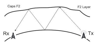
Fig 5.5. Sketch of a 2F radio link.

Using the diagram shown in the figure 5.6 we can calculate the lenght of the radio path.

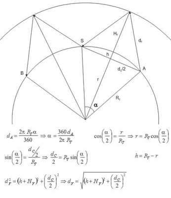
Fig 5.6. Geometry of the link using two hops.

A = Location of the transmitter at Tenerife (Canary Islands).

B = Location of the receiver at Paraíba (Brazil).

S = Middle point of the trajectory transmitter/receiver over the Earth's surface.

dA = Arc length between points A and S.

dC = Chord length between points A and S.

RT = Earth's radius = 6370 km.

HF = Altitude of the reflection points.

dF = Distance from the transmitter to the first reflection point in the ionosphere.

The total length of the radio path is 4 x dF. If we consider that ionospheric reflection occurs at the F layer, being HF = 230 km, and that the distance from A to B is 4536 km, the radio path would have a length of 4701 km.

The figure 5.7 shows the projection of the different reflection points over the Earth's surface.

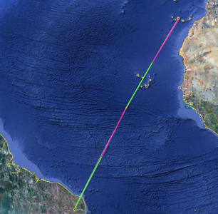
Fig 5.7. Theoretical reflection points in the mode 2F.

The first reflection in the ionosphere would occur at a latitude of 19º and the second one at a latitude of 1º, practically over the Equator.

If we consider an altitude HF = 300 km, the analysis made with BeamFinder [Ref.BeamFinder] shows that the stations in the northeast of Brazil would be inside the shadow area between the first and the second hops, as we can see in the map shown in the figure 5.4.

5.2.2. Power budget.

Considering a radio path length of 4701 km and taking into account free space propagation losses only, the fading margin would be MF = 47,83 dB.

However, the takeoff angle necessary for this geometry would be of 16 degrees, so if the antennas are pointing to the horizon their gain at this angle would be lower, and even lower if the azimuth is incorrect, making this fading margin lower also and perhaps too risky.

5.2.3. Ionospheric conditions.

The first approach consisted on the utilisation of a prediction software (W6ELProp) to simulate the MUF between Tenerife and Paraíba, using the parameters of the days under study. The results are shown in the figure 5.8. As can be seen, the calculated MUF was always below 33 MHz and never reached the 50 MHz band.

Fig 5.8. MUF between Tenerife-Paraíba calculated with W6ELProp

We used also the Proplab map provided by Solar Terrestrial Dispatch, which allows to calculate the approximated values of the MUF for radio links greater than 3000 km. The figure 5.7 shows the map corresponding to 03/21/2010 at 21:55 UTC. The calculated MUF was not higher than 36 MHz in any case.

Fig 5.7. Proplab map used to calculate MUFs

Due to those two facts, and taking into account also that we are currently almost in a minimum of the solar cycle (SSN=33). the 2F mode hyphotesis was initially discarded.

However, once the Tucuman (Argentina) ionosonde data was available, we saw that the MUF(3000)F2 prediction reached values higher than 50 MHz during the time window where some of the contacts took place (see fig.4.5), reviving this way the 2F mode hyphotesis. It is necessary to take into account that this ionosonde is located in Argentina, not in Brazil. Also, the distance of the radio contacts made was higher than 3000 km, so the MUF Tenerife-Paraíba could have been even higher, supporting this way the 2F theory.

Anyway, in the case of other ionosondes in nearest places to the radio path, the MUF(3000)F2 reached maximums of 40 MHz (Fortaleza) and 36 MHz (Sao Luis) when they weren't affected by spreaf-F, that is, near 20:00 UTC. It should be normal that MUF(3000)F2 values were even lower as time advanced, due to lower photoionozation and higher recombination.

In regards of the reflection points in the ionosphere, the first point is very near the ionization peak due to the equatorial anomaly, but the second one is at the minimum between peaks. Although a wave of 50 MHz could be reflected at the first point, something we can doubt about due to the solar cycle and the hour of the day, it would be much less probable for the second reflection to occur.

5.2.4. Discussion.

Aspects for the 2F hyphotesis:

The MUF(3000)F2 predicted by an ionosonde relatively near in Tucuman (Argentina) showed values higher than 50 MHz during the days of the contacts.

Aspects against the 2F hyphotesis:

There is a strong possibility of range spread in the Tucuman ionosonde, so its measurements and predictions could suffer from significative errors.
The MUF between Tenerife and Paraíba predicted with W6ELProp is always below 33 MHz.
The MUF between Tenerife and Paraíba predicted with Proplab is always below 36 MHz.
The MUF(3000)F2 predicted by the ionosondes at Fortaleza and Sao Luis was always below 40 MHz and 36 MHz, respectively.
The fading margin could be too low if the antennas weren't properly pointed in azimuth and elevation.
The second reflection at the ionosphere would occur over the Equator, where there is an ionization minimum due to the equatorial anomaly.

5.3. Complex modes hyphotesis.

The complex propagation modes consist on multiple refractions or reflections in different layers of the ionosphere. The following modes would have a certain possibility to occur:

Mode 1F1E: first hop through the F layer and second hop through the E layer.
Mode 1E1F: first hop through the F layer and second hop through the E layer.
Same modes described above but using the sporadic Es layer instead of the E layer.

5.3.1. Ionospheric conditions.

The radio contacts were established in the evening, so the electron recombination in the ionosphere was suppossed to have started and the E layer to start vanishing, something we have seen in the ionograms. Due to this, the 1F1E and 1E1F modes would be discarded.

In regards of the sporadic E layer, the ionosondes nearest to the radio path (Fortaleza and Sao Luis) show the presence of this layer during several hours of the days, although there is time coincidence with only one of the radio contacts established. On the other hand, although the foEs values (critical frequency of the Es layer) are high, with maximums up to 5,850 MHz (figs. 4.12 and 4.20), it is not clear that they would be high enough to permit reflection of radio waves of 50 MHz with oblique incidence.

However, the area where the second ionospheric reflection would take place in a theoretical 1F1Es is somewhat far of the ionosondes, so we must not discard the possibility of a sporadic E layer over the Atlantic with enough density of ionization to permit reflection at 50 MHz.

In regards of the possible 1Es1F mode, we don't have information about the possible development of an sporadic Es layer between the Canary Islands and the Cape Verde Islands. This zone is within the equatorial anomaly, with an high density of ionization during the day, so in case the Es would have existed, its foEs could have been even higher than the measured by the ionosondes at Brazil, although it is impossible to know whether enough to permit the propagation at 50 MHz. Anyway, the second hop would have took place in the F layer, near the Equator, where the density of ionization is much lower and most probably not enough to permit the propagation at this frequency, mostly considering the current situation of solar minimum.

5.3.2. Discussion.

Aspects for the complex modes hyphotesis:

The possible development, not verified due to the lack of data, of a sporadic Es layer between the Canary Islands and the Cape Verde Islands, could made the mode 1Es1F possible, only in case its density of ionization was high enough.

Aspects against the complex modes hyphotesis:

The E layer had already vanished at the hour of the contacts, thus discarding the 1F1E and 1E1F modes.
The sporadic Es layer registered by the ionosondes at Fortaleza and Sao Luis (Brazil) doesn't seem to have enough density of ionization to permit the reflection of radio waves of 50 MHz with oblique incidence, thus discarding the 1F1Es mode.
The 1Es1F mode doesn't seem to be probable because the second reflection would have taken place at a point very near the Equator, where the density of ionization is lower due to the equatorial anomaly, with regard to higher latitudes and mostly during the solar minimum.

5.4. eTEP hyphotesis.

Taking into account the hour and date of the contacts, one of the most accurate hyphotesis points to evening transequatorial radio propagation (eTEP). All the contacts were made between 21:50 GMT and 22:53 GMT (GMT was y the local time at the Canary Islands), in or around the date of the spring equinox, which seems to be favourable for TEP to occur.

5.4.1. Introduction to the TEP modes.

There are two different modes of transequatorial propagation. The first one is the afternoon TEP (aTEP), which occurs during the afternoon, in conditions of maximum ionization [Ref.Yeh]. As we have seen in the section 2.1, as a consequence of the equatorial anomaly the ionizacion maximum doesn't happen in the region of the ionosphere above the Equator, but at latitudes between 10º and 20º. If the density of ionization is very high (i.e. around the solar cycle maximum), within those ionization peaks refraction of VHF radio waves can occur, as shown in the figure 5.10. If refraction occurs in both peak regions, long distance transequatorial radio links are possible in the indicated bands. This mode is of chordal type and is called FF mode.

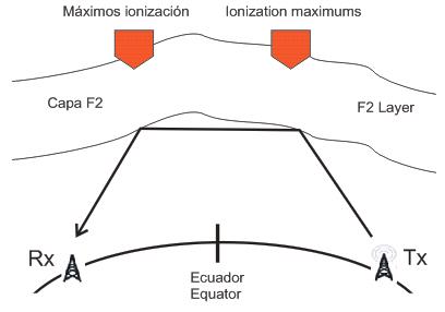
Fig 5.10. Sketch of a aTEP (FF) radio link

The hour of the radio contacts was between 21:50 UTC and 22:52 UTC, so there wasn't aTEP. However, they are within the time window of the other type of transequatorial propagation, called evening TEP (eTEP).

As we have seen in the section 2.2, during the evening, in the equatorial zone and low latitudes, equatorial plasma bubbles (EPB) appear forming field aligned irregularities (FAI): as a result of the dynamic processes of the beginning of electron recombination during the evening, irregular ionization clouds are created, growing with time, moving upwards and vanishing around 03:00 AM. Those clouds are aligned with the geomagnetic field. The gaps in density of ionization between those clouds and the areas less ionized cause refraction and even propagation of radio waves through ducts, increasing their range, as shown in the figure 5.11.

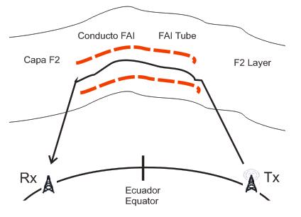
Fig 5.11. Sketch of an eTEP radio link

Those ducts are aligned following the direction of the magnetic North-South (perpendicular to the magnetic Equator) with a maximum deviation of about 15 degrees. The figure 5.12 shows the number of EPBs registered between 1989 and 2000 [Ref.Burke]. The horizontal axis is the geographic longitude and the vertical axis is the number of the day within the year. The number of observed EPBs is represented with the color code. In our particular case, we are between 234º (Paraiba) and 344º (Canary Islands), between the days 77 (03/17/2010) and 81 (03/21/2010), being the probability of EPB events at medium/high level from a statistical point of view.

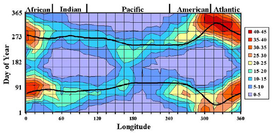
Fig 5.12. Distribution Day-Longitude for the number of EPBs registered between 1989 and 2000.

5.4.2. Geometric analysis.

The peculiarity of the radio contacts under study is that the angle between the radio path and the geomagnetic North-South direction is not within the expected values, as shown in the figure 5.13.

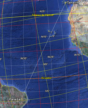
Fig 5.13. Angle of the radio path with the geomagnetic N-S direction.

In the figure, the radio path is represented by a white line, the geographic coordinate system by a red grid and the geomagnetic coordinate system with a yellow grid (thin lines).

We can see that the angle of the radio path with the geomagnetic meridians is 35º at Paraiba and 42º at the Canary Islands, in both cases very far from the theoretical 15 degrees stated for TEP propagation [Ref.TRP] [Ref.Harrison]. This is one of the facts we consider of interest about those radio contacts.

5.4.3. Ionospheric conditions.

The observations point to the formation of equatorial plasma bubbles (EPB), as shown in the ionograms of Ascension Island (fig.4.9), Fortaleza (fig.4.16) and Sao Luis (fig.4.24), revealing range spread during almost all the hours of the radio contacts. Those range spread observations indicate the presence of ionospheric irregularities in the southerner part of the radio path, most probably aligned with the geomagnetic field (FAI). There is no data available for the northern part of the radio path. However, the scintillation maps (fig.4.35-38) reveal scintillation south of the Canary Islands during the hours of the radio contacts.

Thus, we can affirm that during the hours of the radio contacts there were ionospheric irregularities probably due to EPB, which may have formed ducts allowing the propagation of 50 MHz radio waves at long distances through the Equator.

However, those ducts are normally aligned or almost aligned with the N-S geomagnetic lines (fig.2.2), so the radio path would not coincide with the orientation of the ducts, unless there were other type of additional phenomenons causing the appearance of ramifications in an oblique way with respect to the N-S direction. Another possibility would be the development of ducts between different EPBs following the trajectory of the radio path. As was indicated in the section 4.1, the geomagnetic field was inactive (Kp=0) and there weren't events of solar radiation storms.

On the other hand, the formation of those ducts is more typical during the solar cycle maximums, and during the radio contacts we were in the solar minimum (SSN=24-28), although it is remarkable that during those days the ionization seemed to be higher than the expected mean values, as seen in the measurements of foF2 and foEs, and also in the predictions of MUF(3000)F2.

Another possibility of propagation consists on scattering with the equatorial plasma bubbles, as suggested in other studies such as the reception of long distance TV signals in Japan in the 47.5-52.2 MHz band [Ref.Takano].

5.5. 2E/3E/4E hyphotesis.

The 2E/3E/4E hyphotesis has been raised from an analysis made by DF5AI, using his software BeamFinder [Ref.BeamFinder]. According to this hyphotesis, the radio contacts were established using two, three and four reflections in the E layer of the ionosphere, or even in sporadic E layers.

5.5.1. Geometric analysis.

The calculations made for multiple E layer or sporadic E layer hops at an altitude of 105 km, gave the results shown in the figure 5.14.

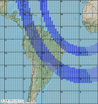
Fig 5.14. Coverage areas for 2E and 3E modes, calculated with BeamFinder (courtesy Volker Grassmann, DF5AI).

The dark blue squares represent the coverage areas for two hops (2E) or three hops (3E) in the E layer or the sporadic E layer, from the Canary Islands. The coincidence with the locations of the stations in Brazil is amazing (fig.3.1). If we extrapolate the results to a possible fourth hop (4E), the stations in Uruguay and Argentina would lay within the coverage area.

Regarding the reflections in the Earth's surface, according to the map shown in fig.5.14 we can see the following for the three reflection points used to complete the 4E mode:

The first reflection in the Earth's surface would be in the Atlantic Ocean, southwest of the Cape Verde archipelago, that is, with an excellent electrical conductivity.

The second reflection in the Earth's surface would be in the northeastern coast of Brazil, around the locations of PT7TT, PT7ZAP, PY0FF, PR7AR and PY7XAF (fig.5.15). The white line crossing diagonally is the radio path between Tenerife (Canary Islands) and Buenos Aires (Argentina). We can conclude that there is reflection also in the Atlantic Ocean, that is, with very good electrical conductivity.

Fig 5.15. Area of the second reflection in the Earth's surface for the 2E/3E/4E modes.

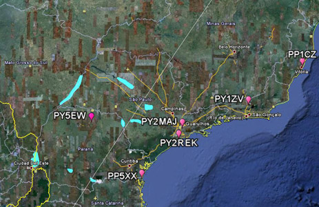
The third reflection in the Earth's surface would be in the inner land of Brazil, around the locations of PP1CZ, PY1ZV, PY2MAJ, PY2REK, PP5XX and PY5EW. The figure 5.16 shows a detail of the area obtained from Google Earth, marking the most significant water masses with blue poligons: Iguaçu River, Itaipu Lake, Parana River, Xavantes Dam, Jurumirim Dam, Barra de Bonita Dam and Promissao Dam. The white line crossing diagonally is the radio path between Tenerife (Canary Islands) and Buenos Aires (Argentina). We can conclude that in this area there are enough water masses to allow the reflection of the radio waves back to the ionosphere.

Fig 5.16. Area of the third reflection in the Earth's surface for the 3E/4E modes.

Regarding the reflections in the ionosphere, they would occur roughly in the regions around the following points:

1st ionospheric reflection: 19.192151°N, 22.833109°W
2nd ionospheric reflection: 1.091503°N, 33.750451°W
3rd ionospheric reflection: 16.702532°S, 44.583789°W
4th ionospheric reflection: 33.935501°S, 57.607773°W

5.5.2. Power budget.

From the point of view of the power budget and using the geometric calculations shown in the fig.5.1, the radio path would have the following lengths (HE = 105 km):

2E mode: 4645 km.
3E mode: 6968 km.
4E mode: 9290 km.

Then we can calculate the fading margin after the losses of propagation only (section 3):

2E mode: MF(2E) = 47,93 dB.
3E mode: MF(3E) = 44,41 dB.
4E mode: MF(4E) = 41,91 dB.

That is, the power budget seems to be enough to allow all the proposed modes.

5.5.3. Ionospheric conditions.

As we have seen in section 4, the ionograms taken near the radio path show the presence of the E layer only in the first samples of each day (until 20:40 UTC maximum), and the radio contacts took place later, so we can expect that at those hours the E layer had vanished. Anyway, some of those ionosondes registered sporadic E layers with critical frequencies up to foEs = 5,900 MHz, that is, quite high. So we must not discard the possibility of sporadic E layers developed at least in 4 areas of the radio path to allow the modes 2E/3E/4E, having enough density of ionization to allow operations in the 50 MHz band.

5.5.4. Discussion.

Aspects for the 2E/3E/4E modes hyphotesis:

The geometry of the links matches perfectly with the locations of the stations contacted.
The power budget seems to be high enough to allow all the proposed modes.
During the contacts, the operators did not feel signal variations which could be associated to scintillation.
The sporadic E layer was registered in areas relatively close to the radio path.

Aspects against the 2E/3E/4E modes hyphotesis:

The E layer had completely vanished at the hours of the radio contacts.

7. References.

[Ref.TRP]
"Transequatorial Radio Propagation".
IPS Radio and Space Services (Australia).

[Ref.Harrison]
"Evening transequatorial VHF propagation".
R. Harrison.

[Ref.Dolukhanov]
"Propagation of Radio Waves".
M. Dolukhanov
Ed.Mir, Moscow (1965).

[Ref.Yeh]
"An Investigation of Motions of the Equatorial Anomaly Crest".
K. C. Yeh, S. J. Franke, E. S. Andreeva, V. E. Kunitsyn (2001).

[Ref.Maruyama]
"Equatorial ionospheric disturbance observed through a transequatorial HF propagation experiment".
T. Maruyama and M. Kawamura.
Annales Geophysicae, 24: 1401-1409 (2006).

[Ref.Burke]
"Seasonal-longitudinal variability of equatorial plasma bubbles".
W. J. Burke, C. Y. Huang, L. C. Gentile, and L. Bauer
Annales Geophysicae, 22: 3089-3098 (2004).

[Ref.Reinisch]
"Multistation digisonde observations of equatorial spread F in South America".
B.W. Reinisch, M. Abdu, I. Batista, G. S. Sales, G. Khmyrov, T. A. Bullett, J. Chau, and V. Rios
Annales Geophysicae, 22: 3145-3153 (2004).

[Ref.BeamFinder]
BeamFinder analysis software: http://www.beamfinder.net/
Dr. V. Grassmann (DF5AI).

[Ref.Pellejero]
"Geometry and operative aspects of the simple modes of ionospheric propagation".
I. Pellejero (EA4FSI)

[Ref.Morgan]
"A Review of VHF Ionospheric Propagation".
Morgan, M.G.
Proceedings of the IRE. Volume: 41 , Issue: 5 (1953). DOI: 10.1109/JRPROC.1953.27439

[Ref.Takano]
"Broadband Observations of Propagation Anomaly of VHF WavesTransmitted from Oversea Broadcasting Stations".
Takano, T.; Sakai, K.; Nagashima, I.; Nakata, H.; Akaike, H.; Ujigawa, S.; Higasa, H.; Shimakura, S.;
IEEE Radio Science Conference, 2004. Proceedings. 2004 Asia-Pacific. DOI: 10.1109/APRASC.2004.1422486

[Ref.Rappaport]
"A Single-hop F2 Propagation Model For Frequencies Above 30 MHz And Path Distances Greater Than 4000 KM".
Rappaport, T.S.; Campbell, R.L.; Pocock, E.;
Geoscience and Remote Sensing Symposium, 1990. IGARSS '90. 'Remote Sensing Science for the Nineties'., 10th Annual Internationa. DOI: 10.1109/IGARSS.1990.688284

8. Glossary.

aTEP: Afternoon TEP.
EPB: Equatorial plasma bubbles.
EEJ: Equatorial electrojet.
eTEP: Evening TEP.
foF2: F2 layer critical frequency.
FAI: Field Aligned Irregularities.
MUF: Maximum Usable Frequency.
MUF(3000)F2: Prediction of the MUF for distances of 3000 km, using hops in the F2 layer.
PCA: Polar Cap Absorption.
SFI: Solar Flux Index.
SSN: Sunspot Number.
TEP: Transequatorial Propagation.
URSI: Union Radio-Scientifique Internationale.

9. Acknowledgements.

Daniel Díaz (EA8DD), provided all the technical data about his radio contacts with Brazil, Argentina and Uruguay.
Alonso Mostazo (EA3EPH), made exhaustive analysis of the ionograms provided by the ionospheric sounding stations near the radio path.

Dr. Volker Grassmann (DF5AI), provided valuable data with his BeamFinder software and on the 2E/3E/4E hyphotesis, and also advice about the contents of this article.

Garth Patterson (IPS Radio and Space Services, Australian Government), provided valuable information about the ionograms analyzed, especially about the range spread events.

Prof. Bodo W. Reinisch (Center for Atmospheric Research, University of Massachusetts Lowell), provided access to the DIDBase database of ionograms.

Ismael Pellejero - EA4FSI
Contact form

EA4FSI-28T1 - Technical Articles

Technical Articles

Other resources

Analysis of the radio contacts between the Canary Islands and South America in the 50 MHz band in March 2010

Table of contents.

1. Introduction.

2. Equatorial ionosphere characteristics.

2.1. Equatorial anomaly.

2.2. Turbulences and FAI.

3. Technical information on the radio contacts.

3.1. Radio contact logs.

3.1.1. EA8BDD's log.

3.1.2. EA8BPX's log.

3.2. Statistical analysis.

3.2.2. Hourly distribution.

3.3. Methodology used in the calculations.

4. Analysis of the ionospheric conditions.

4.1. Space weather conditions.

4.2. Contenido total de electrones (TEC).

4.3. Ionograms.

4.3.1. Tucumán ionosonde.

4.3.2. Ascension Island ionosonde.

4.3.3. Fortaleza ionosonde.

4.3.4. Sao Luis ionosonde.

4.3.5. Cachoeira Paulista ionosonde.

4.4. Ionospheric scintillation maps.

5. Propagation modes hyphotesis.

5.1. One-hop hyphotesis.

5.1.1. Geometric analysis using straight rays.

5.1.2. Analysis using BeamFinder.

5.1.3. Ionospheric parabolic model.

5.1.4. Scattering from regular ionization areas.

5.1.5. Power budget.

5.1.6. Ionospheric conditions.

5.1.7. Discussion.

5.2. 2F hyphotesis.

5.2.1. Geometric analysis.

5.2.2. Power budget.

5.3. Complex modes hyphotesis.

5.4. eTEP hyphotesis.

5.5. 2E/3E/4E hyphotesis.

5.5.1. Geometric analysis.

5.5.2. Power budget.

5.5.3. Ionospheric conditions.

5.5.4. Discussion.

7. References.

8. Glossary.

9. Acknowledgements.