Notes on Antenna Simulation using NEC-2

1. Introduction.

These notes are a collection of recommendations and design rules for performing antenna simulations with programs based on the NEC-2 algorithm. These notes are not intended as a guide to using the various programs based on this algorithm, but rather as a quick reference for users already familiar with their use. The recommendations and design rules have been collected from the user’s manuals of some programs and from technical articles about antenna simulation, with references listed in Section 8.

Failure to comply with the design rules inherent in the NEC-2 algorithm may have a great impact on the simulation results. For example, the resulting calculations of antenna impedance will often be erroneous and the simulated radiation patterns unrealistic.

The NEC-2 algorithm was developed in 1981 in the United States by the Lawrence Livermore National Laboratory, with the sponsorship of the Naval Ocean Systems Center and the Air Force Weapons Laboratory [1] and is based on the method of moments [2].

Note that some of the rules are not applicable to later versions of the algorithm (NEC3 and NEC-4), which are more advanced and whose code is not available to the public. On the other hand, take into account that not all well-known antenna simulation programs available as shareware are based on this algorithm. For example, 4Nec2 and EZNEC are based on NEC-2, but others such as MMANA-GAL are based on variations of MININEC [9].

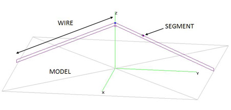
The following terminology will be used throughout this article (see fig.1):

• Model: a simulation setup comprising all the radiators of the antenna (including the loads), the generator and the type of ground.

• Wire: each of the straight conductors forming an antenna model in the programs based on NEC-2. In order to define a wire of length L_h in NEC-2, it is necessary to specify the coordinates of the two points delimiting its ends, the conductive material employed, the wire diameter D_h and the number of segments which will form the wire. Let Z_s be the height of the wire over the ground. If the wire is not parallel to the ground, the height of the end nearest to the ground will be considered. We will denote the number of segments making up a wire by N_s.

• Segment: each straight section into which a wire is divided in an antenna modelled with programs based on NEC-2, used by the algorithm for the computation of currents by means of pulses. The segments will have a length L_s, which may be specified by the user or computed automatically by some of the programs, a process named autosegmentation. The method of moments, on which NEC-2 is based, computes the interactions between segments.

• Segment density: number of segments per wavelength in a wire. Note that in the case of multiband or wideband antennas, the segment density will be different for each working frequency.

• Wavelength (λ): the wavelength corresponding to the working frequency of a specific simulation in a program based on NEC-2.

• Critical zone: a part of a model presenting geometric characteristics which require special design considerations in order for the NEC-2 simulations to be correct.

2. Coordinate system.

Understanding the coordinate system employed in a simulation program is fundamental both for the design of the models and to correctly evaluate the results of the simulations. The coordinate systems may be different among the different programs based on NEC-2. Figure 2 shows the coordinate system used in 4Nec2.

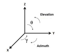
The ground is simulated in the XY plane and the Z axis represents the height over the ground.

The following angles are defined:

• θ: angle measured between the positive Z-axis and the ground plane XY. In this manner, the ground plane may be defined as the plane θ = 90°.

• φ: angle measured between the positive X-axis and the YZ plane.

• Elevation: angle measured between the ground plane XY and the positive Z-axis. An elevation of 90° will correspond to the perpendicular to the ground plane.

• Azimuth: angle measured in planes parallel to the XY ground plane. The azimuth angles are measured clockwise from the Y axis towards the X axis. The Y axis has an azimuth of zero degrees.

2.1. Conventions for model representation.

In order to make possible the comparison of the radiation patterns of different antennas in an easy way, it is advisable to represent all models geometrically according to a set of general conventions. In this section, a set of conventions taken from [5] is shown:

• If the model includes ground, it will be located in the XY plane.

• The Z axis will represent the height of the antenna over the ground plane XY.

• All the linear elements of the antenna will be represented in the Y axis or in other axes parallel to the Y axis.

• The X axis will be used for the front-to-back direction. For isolated elements, we will establish X=0.

• If the model has symmetry, as far as possible the axes of the coordinate system will be used as axes of symmetry.

3. Geometry of the models.

Before defining the structure of a model in NEC-2, it is necessary to consider how current flow is represented in each simulation program. For example, in 4Nec2 positive current always flows from end 1 to end 2 of each wire.

On the other hand, it is necessary to observe the geometric rules presented in the next sections.

3.1. General rules.

In order to avoid errors, it is advisable to observe the following general rules while designing simulation models:

• Two wires must not meet at intermediate points of any of their segments [5].

• In a model with several wires, it is advisable not to connect short segments with long segments [4]. Some programs may impose conditions in this regard. For example, in 4Nec2, for two connected segments “i” and “j” the condition L_si ≤ 5 × L_sj must be fulfilled [7].

• The angle formed by two joined segments, their length and their diameter must be configured in such a way that the central thirds of both segments do not overlap [4, 8].

• Two parallel or nearly parallel wires that are very close to each other must have their segments aligned [3, 4] and must have the same kind of segmentation [7]. It is advisable for the distance between them to be at least several wire diameters as well [8].

• If two wires of different diameters are close of each other, despite the fact that their segments are aligned, errors in the computation of the antenna gain and its input impedance may be obtained, especially in the reactance component [5, 11]. In models with these characteristics it is advisable to perform the AGT test (see section 7.2) in order to check their validity.

• If two wires of different diameters join at a point, the results of the simulations may not be precise [5]. This problem can be minimized by changing the wire diameter in a series of steps through several additional intermediate wires [3].

• NEC-2 allows up to approximately 30 equally spaced radial wires to join at the same point [3], for example in order to simulate a plane of radials. It is not advisable to employ a higher number because the angle between each pair of wires would be small and the results of NEC-2 would lose precision [5].

3.2. Length of the segments.

To improve simulation results, and except in critical zones of the model, it is advisable for all segments in a model to have the same length [4, 5].

Regarding the minimum length of the segments (L_s,min), the references consulted specify the following restrictions related to the wire diameter and wavelength:

• L_s,min > D_h [8]

• L_s,min > 2 × D_h [4]

• L_s,min > 4 × D_h [5]

• L_s,min > λ/10000 [7, 10]

Regarding the maximum segment length (L_s,max), the following restrictions related to the wavelength are specified:

• L_s,max < λ/20 [4, 7] must be observed, at least in critical zones.

• L_s,max < λ/10 [7, 10] is sufficient in most cases; even L_s,max < λ/5 may be used for segments integrated in long wires without critical zones.

3.3. Radius of the wires.

According to our terminology, the wire radius is defined by D_h/2. Restrictions related to the minimum and maximum radius of the wires, as a function of the length of the segments, may be imposed in some programs. For example:

• in 4Nec2, the proportion D_h/2 < L_s/10 must be observed [7].

3.4. Segment density.

Under normal circumstances, the higher the segment density, the better results will be obtained in the simulations, at the cost of increased computation time. Nevertheless, if a model is already precise enough, an increase of the segment density will not provide further improvements.

On the other hand, it is necessary to take into account that if the total number of segments in a model is very high, the maximum number of segments allowed by some programs may be reached [9].

One wire must have at least 8–10 segments per half-wavelength [5, 8]. If this rule is not observed, the results won’t be precise, especially those related to the computation of the input impedance of the antenna. If a wire is a quarter-wavelength long, five segments is a reasonable minimum [5].

In the case of multiband or wideband antennas, the segment density will be different for each working frequency. Therefore, the number of segments employed must be changed with the frequency, or must be calculated in order to be above the recommended minimum corresponding to the highest working frequency (shorter wavelength) [8].

In order to determine the optimum segment density, it is interesting to perform a convergence test (see section 7.1).

4. Types of ground and height of the wires.

In this section, the characteristics of the different types of ground available in most programs implementing the NEC-2 algorithm are described. For each case, specifications are provided regarding whether the wires may touch the ground and, if not, the minimum height at which they must be placed above it.

In every case except free-space simulations, it is necessary to take into account the diameter of the wires: the minimum height of a horizontal wire over the ground must be at least twice the diameter of that particular wire:

• Z_s > 2 × D_h [4]

4.1. Free space.

In free-space simulations, there is no ground plane. Normally, the results will be similar to those one may find in the textbooks.

4.2. Perfect ground.

Perfect ground consists of a perfectly conducting ground plane, without losses. It is advisable to perform simulations with ground losses omitted in order to assess their influence on the results by comparison with further simulations using more realistic ground types.

Model wires may touch perfect ground.

4.3. Fast ground.

With the fast ground type, NEC-2 uses a method based on complex reflection coefficients.

The wires of the model cannot touch the fast ground.

Horizontal wires must be placed at least one tenth of the working wavelength above the ground.

• Z_s > λ/10 [4, 8] for horizontal wires.

4.4. MININEC ground.

The MININEC ground model assumes a perfect ground for the computation of the currents and changes to a dielectric ground for the computation of the far field patterns (ground without losses). With the MININEC ground, hybrid calculations designed for the first generation of less powerful computers are used.

The vertical wires can touch the MININEC ground.

The horizontal wires cannot touch the ground. They must be placed at a height over the ground of at least one fifth of the working wavelength:

• Z_s > λ/5 [4, 8] for horizontal wires over MININEC ground.

If this rule is not observed, the simulations with NEC-2 will produce erroneous impedances and anomalously high gains, especially for horizontal polarization.

4.5. Sommerfeld-Norton (S-N) ground.

The Sommerfeld–Norton (S-N) model is the most accurate ground model, with the highest computational cost and is the best method to simulate horizontal wires very close to the ground.

When using S-N ground, both vertical and horizontal wires must not touch the ground.

One way to simulate a connection of a vertical wire to the ground is by means of a virtual plane of at least eight radials [7], taking into account that the electrical conductivity characteristics of the simulated ground will be modified and therefore that the results may be inaccurate.

In the references consulted, the following rules related to the height of the horizontal wires have been found:

• Z_s > λ/200 [4]

• Z_s > λ/1000 [5, 8]

5. Generators, loads and transmission lines.

This section presents recommendations and design rules about the characteristics of the generators, loads and transmission lines to be used in the simulations.

The loads and transmission lines used in NEC-2 are mathematical models instead of physical models. Therefore, they do not contribute to the radiation of the antenna [5, 8]. If the transmission line is expected to influence the radiation of the actual antenna, it is possible to try to create a model of the line in some particular cases, such as with the parallel transmission line.

As a general rule, a generator of complex value 1 +j0 will be adequate for most of the simulations [4, 5]. In the simulation of arrays, it may be necessary to use several phase-shifted generators. See an example in the article “Adcock/Watson-Watt Radio Direction Finding”.

Take into account that generators or loads must not be placed at the ends of open-circuit wires [7, 11]. The generator would see a load at one terminal and an open circuit at the other, so theoretically no current would flow. In the simulations, the input impedance of the antenna would be erroneous, reaching too high values (especially in the reactive part) and only a very low current would be induced through the mutual coupling between the part of the generator connected to the antenna and the piece of segment connected to the other pole of the generator, which remains in open circuit.

If the generator is to be placed in the center of a wire, it is recommended to model this wire with an odd number of segments [5], so there will be a symmetrical distribution of currents in the wire.

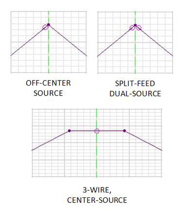
If a generator is to be placed in the apex formed by two wires joining with an angle different from 180°, such as in the case of inverted-vee antennas, several techniques can be used [3, 5, 6, 8, 10] as shown in Figure 3.

• Off-center source: the least precise option consists in placing only one generator in one of the wires. The distribution of currents may be asymmetric and the values of the input impedance of the antenna may be inaccurate. The precision may be improved using the technique of “segment tapering”, dividing each wire into several concatenated wires and using shorter segments in the wires closest to the generator, in a way that the generator is placed close to the apex.

• Split-feed / Dual source: this technique consists of using two generators (one on each of the final segments of the wires joining in the apex) of half the voltage which would be used with only one generator. It is interesting to configure a high segment density so that the generators are very close to the apex.

• 3-wire, center source: finally, the most precise technique consists in joining both wires with a third additional small wire with three segments and placing the generator in the central segment of the latter. This is the most precise technique for accurately simulating antenna impedance, provided that the length of the three segments of the additional wire is similar to the length of the segments of the two main wires.

6. Other considerations.

This section presents additional recommendations and design rules not related to the previous sections:

• The method of moments [2] is adequate for the simulation of antennas with thin wires. The simulation of thick wires may be problematic, especially in the VHF/UHF bands [8].

• NEC-2 lacks the capacity to model dielectrics, such as underground radials or antennas with electrically isolated wires (twin-lead J-pole, twin-lead folded dipole) [4].

• Take into account that NEC-2 computes the total current in the antenna, without distinguishing between common-mode and differential-mode currents [4].

• In all the radiation patterns calculated with NEC-2, the gain is expressed in dBi.

• NEC-2 does not allow underground wires to be modelled [5, 11].

• NEC-2 is not adequate to model small loop antennas (circumference less than 0.05 λ) because in the simulations the calculated input impedance of the antenna may be zero or negative [11].

7. Model verification.

Once the model has been defined, some programs implementing the NEC-2 algorithm provide options for geometric validation to detect unconnected wires or incorrect crossings, as well as segment validation options to verify whether the rules described in the previous sections are observed. It is advisable to perform both validations before continuing with the convergence and average gain tests.

In the case of wideband or multiband antennas operating between a minimum frequency F_min and a maximum frequency F_max, I suggest the following design strategy, for example with the help of a spreadsheet:

• Once the geometry of the antenna is defined, number the wires, identifying also their diameter D_h(i) and their length L_h(i). For each of the wires “i”, perform the tasks described below.

• Considering the frequency F_min, compute the lengths L_s,min(F_min) and L_s,max(F_min) for the segments of that particular “i” wire (see section 3.2), considering whether the wire will be in a critical zone or not as well.

• Considering the frequency F_max, compute the lengths L_s,min(F_max) and L_s,max(F_max) for the segments of that particular “i” wire (see section 3.2), considering whether the wire will be in a critical zone or not as well.

• For F_min, determine the minimum number of segments N_min(F_min), taking into account both the segments-per-half-wavelength criterion and the calculation L_h(i)/L_s,max(F_min).

• For F_min, determine the maximum number of segments N_max(F_min), calculating L_h(i)/L_s,min(F_min).

• For F_max, determine the minimum number of segments N_min(F_max), taking into account both the segments-per-half-wavelength criterion and the calculation L_h(i)/L_s,max(F_max).

• For F_max, determine the maximum number of segments N_max(F_max), calculating L_h(i)/L_s,min(F_max).

• The number of segments allowed for the “i" wire, N_s(i), must lie within the range [N_min(F_max), N_max(F_min)]. Determine the optimum final value by performing the convergence test described in the next section.

In order to check the validity of a model, it is recommended to perform both the convergence test and the average gain test. Using only one of these tests does not ensure that the model is valid [8].

7.1. Convergence test.

The convergence test can be used to determine the optimum number of segments to be used in a particular model.

It consists of running several simulations of the same model, increasing the number of segments by 50% (a smaller increase if necessary to comply with the geometric rules) on each simulation and making a note of the maximum gain and the input antenna impedance at each step. The optimum segmentation level will be achieved at the step where no significant changes in both parameters are seen [5, 8]. Once this point has been reached, it doesn’t make sense to use a higher number of segments because the results won’t be improved and additional computation time will be required.

For each configuration of number of segments to be tested, perform a segment validation test with your program before making the convergence test.

In the case of wideband or multiband antennas, make the convergence test only with segment-count configurations that lie within the limits computed in the previous sections. It doesn’t make sense to test other different configurations because geometric errors would occur. Before making the convergence test with each possible configuration of number of segments, perform segment validation at the minimum and maximum frequencies of the antenna’s working band, as a double precaution to avoid problems with the geometric rules. The convergence test must be repeated in a representative set of frequencies across the entire operating band of the antenna. Depending on the test results, it is possible to reach a situation where different configurations of number of segments for different sets of frequencies within the working band of the antenna must be used in the simulations.

7.2. Average gain test (AGT).

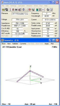
The average gain test is a useful tool to check the validity of a model and it is available in virtually all programs implementing NEC-2. See Figure 4.

The AGT consists in placing the model, without loads and transmission lines, in free space (horizontal antennas) or over perfect ground (vertical antennas) and then to simulate the 3D radiation pattern.

In theory, the average gain of a lossless antenna, considering an adequate sampling over all possible radiation directions, must be equal to 1. That is, the antenna must radiate all the power supplied by the generator [5, 8]. If this rule is not observed, the model probably has defects in the specifications of the generator or the generator may be incorrectly positioned.

The AGT results are interpreted as follows [7]:

• AGT < 0.80: the model is questionable and should be refined.

• 0.80 ≤ AGT < 0.90: the model may be useful, but can be improved.

• 0.90 ≤ AGT < 0.95: the model is usable for most purposes.

• 0.95 ≤ AGT < 1.05: the model is likely to be accurate.

• 1.05 ≤ AGT < 1.10: the model is usable for most purposes.

• 1.10 ≤ AGT ≤ 1.20: the model may be useful, but can be improved.

• AGT > 1.20: the model is questionable and should be refined.

In the case of wideband or multiband antennas, repeat the convergence test in a representative set of frequencies across the antenna’s entire operating band.

8. References.

1. G. J. Burke and A. J. Poggio, Numerical Electromagnetics Code (NEC)—Method of Moments, Part II: Program Description—Code, Rep. UCID-18834, Lawrence Livermore Laboratory, Jan. 1981. [Online]. Available: NEC-2 Part II.

2. R. P. Haviland, W4MB, “Programs for antenna analysis by the method of moments,” in The ARRL Antenna Compendium, vol. 4. Newington, CT, USA: ARRL, 1995, pp. 69–73.

3. G. J. Burke and A. J. Poggio, Numerical Electromagnetics Code (NEC)—Method of Moments, Part III: User’s Guide, Rep. UCID-18834, Lawrence Livermore Laboratory, Jan. 1981. [Online]. Available: NEC-2 Part III.

4. S. D. Stearns, K6OIK, “Antenna modeling for radio amateurs,” presented at the ARRL Pacificon Antenna Seminar, San Ramon, CA, USA, Oct. 2008. [Online]. Available: K6OIK presentation archive.

5. L. B. Cebik, W4RNL, “A beginner’s guide to modeling with NEC,” Parts 1–4, QST, Nov. 2000–Feb. 2001, pp. 34–38, 40–44, 44–48, and 31–35, respectively. [Online]. Available: ARRL Antenna Modeling.

6. L. B. Cebik, W4RNL, “Dipoles: Variety and Modeling Hazards 1. Linear, V, and Folded Dipoles in NEC,” Antenna Modeling, no. 108, AntenneX. [Online]. Available: Cebik archive.

7. A. Voors, 4Nec2 General Help. [Online]. Available: 4Nec2.

8. “Antenna Modeling & System Planning,” in The ARRL Antenna Book, 21st ed. Newington, CT, USA: ARRL, 2010, ch. 4, pp. 4-1–4-18.

9. R. Lewallen, W7EL, “MININEC: The other edge of the sword,” QST, vol. 75, no. 2, pp. 18–22, Feb. 1991.

10. L. B. Cebik, W4RNL, “V Arrays and Beams,” Long-Wire Antennas, Part 3, AntenneX Online Magazine, Jul. 2006. [Online]. Available: Cebik archive.

11. R. Lewallen, W7EL, EZNEC v. 5.0 User Manual. [Online]. Available: EZNEC v. 5.0 User Manual (PDF).