Adcock/Watson-Watt Radio Direction Finding

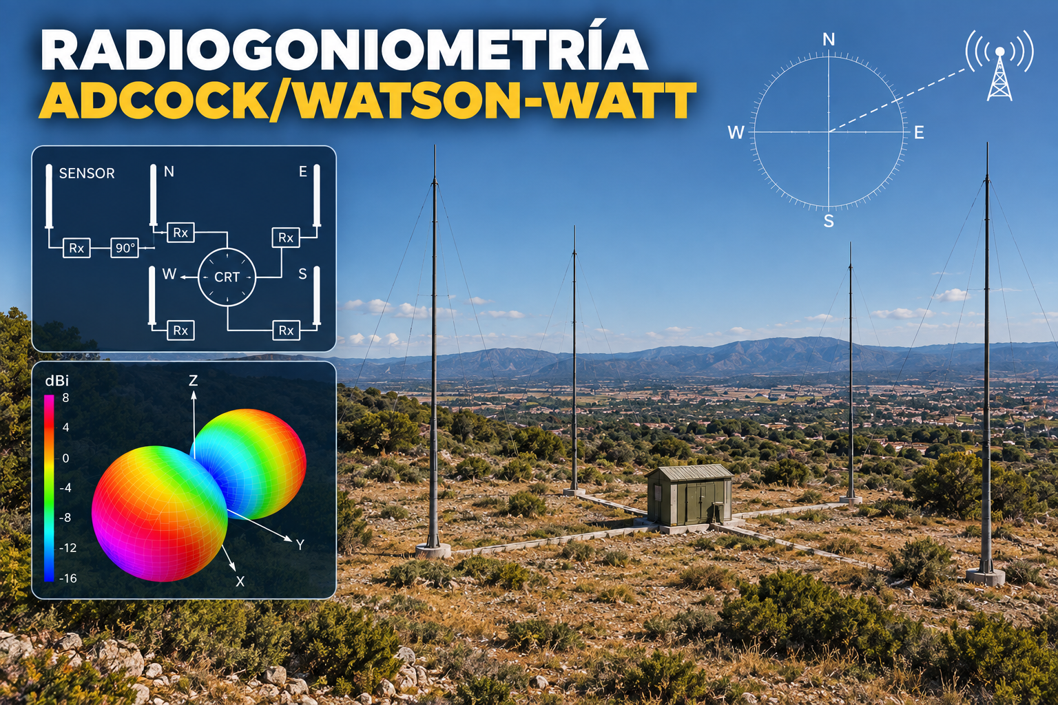
“It has for some time been recognized that the wireless operator employed at a D/F station must be regarded as a specialist, and experience has shown the necessity for specialized training of those who are to undertake this work.”W. E. Crook · D/F Handbook for Wireless Operators · 1942

1. The Adcock array and the Watson-Watt system.

During the Second World War, one of the most common techniques of radio direction finding employed in the “Y” stations for signals intelligence¹ (SIGINT) was based in the use of arrays of 4 monopoles or dipoles arranged in an orthogonal pattern². By means of rotating the array and combining the signals received in a proper way, a bidirectional radiation pattern is achieved, allowing the direction of arrival to be determined of a radio signal of interest, especially through the nulls of the radiation pattern³. This technique was patented by the Lieutenant Engineer Frank Adcock, No.3 Army Wireless Observation Group, in 1919⁴. This is therefore a method of amplitude comparison to determine the direction of arrival of radio signals (DF, Direction Finding)⁵.

In an Adcock array, the four antennas are grouped in pairs, laying each pair along a reference axis. Suppose, for example, that one pair lies in the North-South axis (Y) and the other lies along the East-West axis (X), as shown in the fig.1.

**Fig.1.** Adcock 4-monopole array simulated in 4Nec2

In 1925-26, Sir Robert Watson-Watt (one of the pioneers of the implementation of radar as an early warning system during World War II) improved the system proposed by Adcock by using a fifth antenna to avoid the ambiguities and using a cathode ray oscilloscope to plot the angle of arrival³, allowing to operate the antenna array in static configuration.

The accuracy of an Adcock/Watson-Watt radio direction finding system in the computation of angles of arrival is estimated to be approximately 2–3 degrees⁶. On the other hand, the system is not adequate for high frequency radio direction finding (HF/DF) for NVIS signals, due to the fact that the radiation patterns of the monopoles or dipoles employed have low gain for high takeoff angles⁷.

In order to back the explanation of the Adcock/Watson-Watt radio direction finding technique from a theoretical point of view, I will use several simulations made with the 4Nec2 software.

In the examples, the aim will be focused on the determination of the direction of arrival (DOA) of a radio signal of interest in the 2–10 MHz range (MF-HF). A specific example for a 5 MHz signal will be shown.

In order to simulate the Adcock array with 4Nec2, I will consider 1/4 wavelength monopoles for a working frequency of 5 MHz. That is, each monopole will have a length of 15 metres. In order to simplify the analysis, the part relative to the antenna coupling in all the working band will be obviated, although in fact the antennas need not be resonant at the frequency of the signal of interest⁸.

The antenna separation or baseline is another important point and must be half the wavelength of the maximum working frequency^9,10 at the most, ideally around 1/8 or 1/10 of the working wavelength^5,7. If the separation is greater than half a wavelength, a risk of having ambiguities in the measurements exists. That’s the reason why, if the bandwith to be watched is high, it may be appropriate to have different lines of base for each frequency range.

In our examples this limit is 10 MHz, with a wavelength of 30 metres, so we will lay each pair of antennas with a separation of 15 metres.

A model of perfect ground will be used, in such a way that it should not be necessary to configure a network of radials to simulate the ground plane of each monopole, according to the NEC-2 algorithm rules of design.

Below you will find the contents of the simulation file. Please note that in the 4Nec2 simulations I will analyze only one of the pairs of monopoles, specifically the N-S pair.

CM 4-monopole Adcock array optimized for 5 MHz
CM by EA4FSI
CM
CE
SY monlen=15 'Monopole length
SY monsep=15 'Monopole separation
GW 1 128 0 monsep/2 0.001 0 monsep/2 monlen 2mm 'North Monopole
GW 2 128 0 -monsep/2 0.001 0 -monsep/2 monlen 2mm 'South Monopole
GW 3 128 -monsep/2 0 0.001 -monsep/2 0 monlen 2mm 'West Monopole
GW 4 128 monsep/2 0 0.001 monsep/2 0 monlen 2mm 'East Monopole
GE 1
GN 1
EK
EX 0 1 1 0 1 0 0 'Generator at North Monopole
EX 0 2 1 0 -1 1.22e-16 0 'Generator at South Monopole
FR 0 0 0 0 5 0
EN

2. Computation of the angle of arrival.

Once the array is configured with each pair of antennas aligned along the N-S and E-W axes, let’s suppose that we start to receive a signal of interest (SOI) whose wavefront arrives at the array with an unknown direction of arrival (DOA), which we need to determine.

Let “Phi” be the angle formed by the direction of propagation of the wavefront of the signal of interest and the E-W axis (the X axis in our reference system). That is, “Phi” is the DOA which we need to compute.

The wavefront will arrive at different times at each of the antennas of the array because the travel distance is different, as shown in the fig. 2. This implies that each antenna will receive the signal of interest with some phase shift.

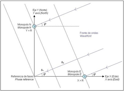
**Fig.2.** Wavefront arrival at the Adcock array

In order to make the computations easier, we will consider the origin of the coordinate system as the phase reference and we will be focused on the first quadrant (N and E monopoles). Each monopole is placed at a distance R from the origin of the coordinate system.

According to the sketch shown in the fig.2, the wavefront arriving at the N monopole travels a distance d1 lower than the distance to the phase reference, whereas the wavefront arriving at the E monopole travels a distance d1+d2 lower. Once these distances are known, we will be able to determine the phase shift of the wavefront in both monopoles

Using trigonometry, we can compute the distance d1+d2 as follows [1]:

\cos (φ) = \frac{d_{1} + d_{2}}{R} \Rightarrow d_{1} + d_{2} = R \cos (φ)

[1]

In a similar way, we compute the distance d1 [2]:

\cos (90 - φ) = \frac{d_{1}}{R} \Rightarrow d_{1} = R \cos (90 - φ) = R \sin (φ)

[2]

Due to the fact that our array is symmetric and having the phase reference at the origin of coordinates, in the S monopole we will have the same phase shift as in the N monopole, buth with negative value. Similarly, at the W monopole we will have the same phase shift as in the E monopole, with negative value.

Therefore, the wavefront will induce the following voltages in each of the monopoles [3]:

\begin{matrix} r_{N} (t) = m (t) e^{j k R \sin (φ)} \\ r_{S} (t) = m (t) e^{- j k R \sin (φ)} \\ r_{E} (t) = m (t) e^{j k R \cos (φ)} \\ r_{W} (t) = m (t) e^{- j k R \cos (φ)} \end{matrix}

[3]

where m(t) is the modulated signal of interest received in the array and K the wave number for the working frequency [4]:

k = \frac{2 π}{λ}

[4]

This wave will have a linear polarization which will probably be neither vertically nor horizontally polarized with respect to the ground plane, due to the effects of ionospheric propagation. Due to the fact that the monopoles of our array are vertical (perpendicular to the ground plane), only the vertical polarization component of the incident wave is considered. The horizontal polarization component, whose energy may cause errors in the determination of the angle of arrival^3,6,8, is eliminated in this way.

At this point, the technique described by Adcock to determine the DOA lies in substracting the signals received in the monopoles of each pair. First of all, let’s consider the subtraction of the signals from the monopoles N and S [5]:

r_{N} (t) - r_{S} (t) = m (t) [e^{j k R \sin (φ)} - e^{- j k R \sin (φ)}]

[5]

Now, we may use the following identity [6]:

\sin (x) = \frac{1}{2 j} (e^{j x} - e^{- j x})

[6]

Expanding expression [5] follows in this way [7]:

r_{N} (t) - r_{S} (t) = m (t) 2 j \sin [k R \sin (φ)]

[7]

On the other hand, we may consider that the wave number K has a very low value for the frequencies in our working band, so finally we can make the following approximation [8]:

r_{N} (t) - r_{S} (t) \approx m (t) 2 j k R \sin (φ)

[8]

Let’s now consider the subtraction of the signals received at the monopoles E and W [9]:

r_{E} (t) - r_{W} (t) = m (t) [e^{j k R \cos (φ)} - e^{- j k R \cos (φ)}]

[9]

Using the identity [6] again, results in [10]:

r_{E} (t) - r_{W} (t) = m (t) 2 j \sin [k R \cos (φ)]

[10]

Similarly, taking into account the small value of the wave number K, we make the following approximation [11]:

r_{E} (t) - r_{W} (t) \approx m (t) 2 j k R \cos (φ)

[11]

In order to determine the DOA, it suffices to calculate the arctangent of the ratio of the two difference signals [8, 11], in the following way [12]:

\arctan [\frac{r_{N} (t) - r_{S} (t)}{r_{E} (t) - r_{W} (t)}] = \arctan [\frac{m (t) 2 j k R \sin (φ)}{m (t) 2 j k R \cos (φ)}] = \arctan [\frac{\sin (φ)}{\cos (φ)}] = φ

[12]

3. Implementation of the method.

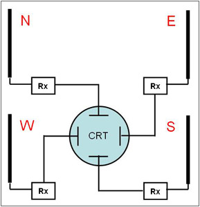
In the first implementations of the method described before, cathode ray tubes (CRT) of the oscilloscope type were employed^3,8. In this type of CRT, the signals plotting in the screen are controlled horizontally by means of applying an electrical field in the plates located in the right and left parts of the device, and vertically by means of another pair of plates placed above and below the screen.

The signals are demodulated in the different receivers or in a single multi-channel receiver. Then, the demodulated signals from the North and South monopoles are applied to the vertical plates and the signals from the East and West monopoles are applied to the horizontal plates, as shown in Fig. 3.

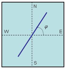
**Fig.3.** Implementation of the method using a CRT

This way, when detecting a signal of interest arriving at the array with a direction of arrival “Phi”, a straight line would be displayed on the CRT, as shown in the fig.4. If the channels N-S and E-W are not well balanced, there will be errors in the DOA computation and an ellipse will be plotted in the CRT, instead of a straight line. It is important to have a correct synchronisation between the local oscillators of the different channels or, even better, to have a common local oscillator⁸.

Knowing the geographical location of several Adcock arrays, the exact position of a transmitter of interest (PF, Position Fixing) can be determined by triangulation using measurements from several stations, using triangulation.

4. Resolving the ambiguity problem

The radiation pattern resulting from the subtraction of the voltages induced in two monopoles has a figure-eight shape^3,5,6,8,11, as shown in the fig.5, obtained from simulations using 4Nec2.

As indicated before, to make the simulations of the diagram with 4Nec2, a source connected to the N monopole and another source connected to the S monopole, with a 180 degree phase shift, have been considered. This way, the simulation of the subtraction of the signals is achieved.

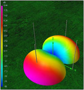
**Fig.5.** Radiation pattern of a pair of Adcock monopoles

The problem of ambiguity, following the previous example, results from a signal arriving at the array with the same angle but from the third quadrant (from the SW) instead of from the first quadrant (from the NE), which may generate the same straight line in the CRT. The same ambiguity will exist between signals arriving with the same angle through the second and fourth quadrants.

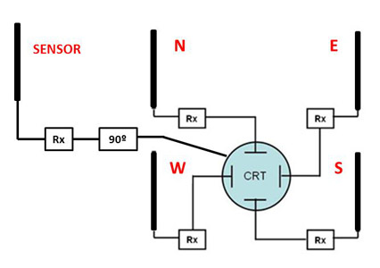
There are several methods to solve the ambiguity problem. The most common of them is adding a fifth antenna, which will be named sense monopole, at the centre of the Adcock array¹¹. The signal received by this additional antenna can be used to modulate the intensity channel of the CRT, by means of plotting the half straight line corresponding to the quadrant where the signal of interest is arriving through. The array layout will be the one shown in the fig.6.

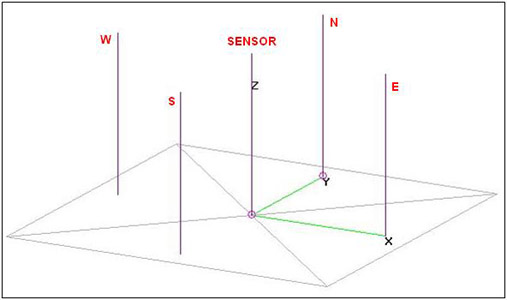
**Fig.6.** Four element Adcock array with sense antenna

This new sense monopole is placed exactly in the phase reference used in our analysis (see fig.2). In order to explain how the system works, we will consider as an example the two following signals of interest arriving at the array:

1) Sinusoidal signal of 5 MHz arriving through the NE quadrant with DOA = 60º (Azimuth = 30º).
2) Sinusoidal signal of 5 MHz arriving through the SW quadrant with DOA = 240º (Azimuth = 210º).

Being in both cases the wavelength equal to 60 m and the wave number [13]:

K = \frac{2 π}{λ} = \frac{2 π}{60} = 0.104719755

[13]

Those two signals would produce exactly the same straight line in the CRT using a system of four monopoles only, that is, a case of ambiguity would occur.

Let’s see what happens when adding the sense monopole.

According to [2], we compute the distance d1 [14]. Recall that the monopoles of the example have a separation of 15 metres between them, so R = 7.5 m:

d_{1} = R \sin (φ) = 7.5 \cdot \sin (60 °) = 6.49 m

[14]

Knowing this distance, the phase shift in the N monopole is [15]:

θ_{N} = K d_{1} = 0.104719755 \cdot 6.49 = 0.679631 rad

[15]

Similarly, according to [1], the phase shift in the S monopole will be −0.679631 rad.

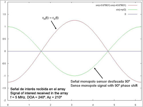
Let’s consider now the subtraction of the signals of the monopoles N-S, as described in [5]. If the wavefront is arriving through the first quadrant (NE), after the process of demodulation we will have the signals shown in the fig.7.

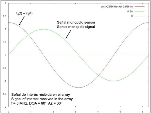
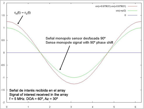
**Fig.7.** Subtraction of the signals N-S and signal in the sense monopole (DOA=60º)

Now, we will shift the phase by 90 degrees of the signal received in the sense monopole, as shown in the fig.8. Note that, with this modification, the zero-crossings occur just at the same time instants.

**Fig.8.** Subtraction of signals N-S and signal in the sense monopole with 90º phase shift (DOA=60º)

Let’s consider now another signal arriving in the opposite direction, through the third quadrant (SW). Using the sense-monopole signal phase-shifted by 90 degrees, we will have the signals shown in the fig.9.

**Fig.9.** Subtraction of signals N-S and signal in the sense monopole with 90º phase shift (DOA=240º)

The results would be similar if we compare signals arriving with equal angles through the quadrants NW and SE.

Analyzing both results (figs. 8 and 9), we conclude that we may use the signal of the sense monopole phase shifted 90 degrees in order to control the plotting of the straight line in the CRT. If we use the positive half-cycles (positive voltage) to enable the plotting in the CRT and the negative half-cycles (negative voltage) to stop it, we will have the two following cases:

If the signal arrives through the NE or the NW quadrants, the voltage applied to the Y axis of the CRT will always be positive and thus only the Y > 0 part of the straight line will be plotted.

If the signal arrives through the SE or the SW quadrants, the voltage applied to the Y axis of the CRT will be always negative and thus only the Y < 0 part of the straight line will be plotted.

Therefore, using this method the ambiguity is solved and only an angle of arrival is determined.

The complete system has the block diagram shown in the fig.10.

**Fig.10.** Block diagram of an Adcock/Watson-Watt radio direction finder with sense antenna

At present, the systems are implemented with digital technology. The signals coming from the receivers are digitized and processed in the time and frequency domains to compute the phase shift, allowing the direction of arrival to be calculated. Besides, using automatic antenna switches, the number of receivers required can be reduced.

5. References and bibliography.

G. Pidgeon, “Bletchley Park—Admiral Sinclair’s War Station,” in The Secret Wireless War: The Story of MI6 Communications 1939–1945. Arundel Books, 2008, pp. 48–54.
P. J. D. Gething, “Review of DF Techniques,” in Radio Direction Finding and Superresolution, 2nd ed., IEE Electromagnetic Waves Series 33. Peter Peregrinus Ltd., 1991, pp. 7–9.
H. D. Kennedy and R. B. Woolsey, “Direction-Finding Antennas and Systems,” in Antenna Engineering Handbook, 3rd ed., R. C. Johnson, Ed. New York, NY, USA: McGraw-Hill, 1993, ch. 39.
F. Adcock, “Improvements in Means for Determining the Direction of a Distant Source of Electro-magnetic Radiation,” British Patent GB 130490, Aug. 7, 1919. [Online]. Available: GB130490A patent record.
H. D. Kennedy and R. B. Woolsey, “Direction Finding Antennas and Systems,” in Antenna Engineering Handbook, 4th ed., J. L. Volakis, Ed. New York, NY, USA: McGraw-Hill, 2007, ch. 47.
E. A. Laport, Radio Antenna Engineering. New York, NY, USA: McGraw-Hill, 1952, pp. 60–67 and 214–215.
A. Rembovsky, A. Ashikhmin, V. Kozmin, and S. Smolskiy, “Direction Finding of Radio Emission Sources,” in Radio Monitoring: Problems, Methods and Equipment. New York, NY, USA: Springer, 2009, pp. 237–316, doi: 10.1007/978-0-387-98100-0.
J. J. Carr, “Antennas for Radio Direction Finding (RDF),” in Practical Antenna Handbook, 4th ed. New York, NY, USA: McGraw-Hill, 2001, ch. 23, pp. 439–456.
U.S. Army Intelligence Center, Introduction to Radio Direction Finding, Subcourse IT0302, ed. C. Fort Huachuca, AZ, USA, Aug. 1999.
J. J. Keaveny, “Analysis and Implementation of a Novel Single Channel Direction Finding Algorithm on a Software Radio Platform,” M.S. thesis, Dept. Electrical and Computer Engineering, Virginia Polytechnic Institute and State University, Blacksburg, VA, USA, Feb. 2005. [Online]. Available: Virginia Tech repository record.
L. Tetley and D. Calcutt, “Radio Direction Finding,” in Electronic Navigation Systems, 3rd ed. Oxford, U.K.: Butterworth-Heinemann, 2001, pp. 346–368.