1. Rhombic antenna.

In this section we will consider the design and simulation of a rhombic antenna terminated in open circuit, without loads of any kind. As we will see, the result is a bidirectional antenna.

1.1. Design of the antenna.

Rhombic antennas are made of two V-shaped wire sections joined at their ends, terminated in an open circuit. Each side of the antenna is made of two legs of length "L" and as a whole the antenna has the shape of a rhombus, that is, the opposite angles are of the same value (Fig. 1).

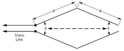
Fig. 1. Rhombic antenna. The ARRL Antenna Book, Chapter13, 20th Ed.

As we will see later, the value of "L" must be an integral number of half wavelengths at the design frequency. The antenna is fed at the vertex opposite the open-circuit end.

1.2. Antenna modelling using 4NEC2.

In order to simulate the antenna in 4NEC2, we will use the geometry shown in Fig. 2. The feed point and the opposite open-circuit vertex lie on the Y-axis, while the other two vertices lie on the X-axis.

We will use the following variables:

L = side length (metres).
A = acute angle of rhombus (degrees).
H = height of installation (metres).

Fig. 2. Model of the rhombic antenna.

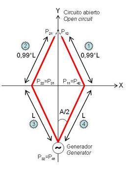
We will define four wire segments as shown in the figure, with the following endpoints (P) and their corresponding coordinates:

Leg #1: P₁₁ (x₁₁, y₁₁) – P₁₂ (x₁₂, y₁₂).
Leg #2: P₂₁ (x₂₁, y₂₁) – P₂₂ (x₂₂, y₂₂).
Leg #3: P₃₁ (x₃₁, y₃₁) – P₃₂ (x₃₂, y₃₂).
Leg #4: P₄₁ (x₄₁, y₄₁) – P₄₂ (x₄₂, y₄₂).

Segments 1 and 2 are reduced 1% in order for this side to become an open circuit.

Using trigonometry, the coordinates of the endpoints of segment 1 will be:

sin(A2) = x₁₁L → x₁₁ = L · sin(A2) y₁₁ = 0

sin(A2) = x₁₁ − x₁₂0.99 · L → x₁₂ = x₁₁ − 0.99 · L · sin(A2) = 0.01 · L · sin(A2)

cos(A2) = y₁₂0.99 · L → y₁₂ = 0.99 · L · cos(A2)

The coordinates of segment 2 are:

x₂₁ = −x₁₂ y₂₁ = y₁₂

x₂₂ = −x₁₁ y₂₂ = 0

Using trigonometry again, the coordinates of segment 3 are:

x₄₁ = 0 y₄₁ = y₃₂

x₄₂ = x₁₁ y₄₂ = 0

And finally, the coordinates of segment 4 are:

x₃₁ = x₂₂ y₃₁ = 0

x₃₂ = 0 cos(A2) = |y₃₂|L → y₃₂ = −L · cos(A2)

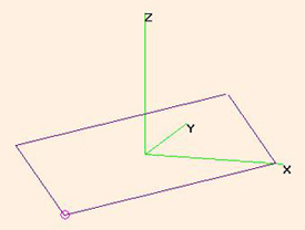
We will assume a design frequency of 14 MHz (21.42 m wavelength). Recall that "L" must be an integral number of half wavelengths at the design frequency. We will therefore choose L = 21.42 m and A = 62°. With those parameters and a scenario of free space, the antenna model in 4NEC2 is shown in Fig. 3.

Fig. 3. Rhombic antenna model in 4NEC2.

Antena_Rombica.nec

1.3. Standing wave ratios.

Having the variables initialized according to the values shown in the previous section, at a frequency of 14 MHz the simulated SWR is 13.2, referenced to 300 Ω.

Fig. 4. SWR referenced to 300 Ω for a rhombic antenna in free space, L=21.42 m and A=62°.

Fig. 4 shows the simulation results for all the HF band (3-30 MHz), using the same parameters. We can see that, in most of the HF band, the antenna could be easily tuned. The SWR is lower at the highest frequencies.

1.4. Radiation patterns.

Fig. 5 shows the radiation pattern of the same antenna in free space, at a frequency of 14 MHz.

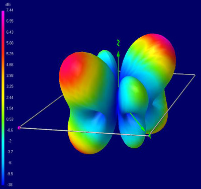
Fig. 5. Rhombic antenna in free space, F=14 MHz, L=21.42 m and A=62°. 3D radiation pattern.

The antenna is bidirectional, with two main lobes along the Y-axis and two secondary lobes along the X-axis. Its maximum gain is 7.44 dBi, and the main lobes have an elevation angle of approximately 45°.

2. Terminated rhombic antenna.

In order to achieve a directive antenna, we will replace the open circuit with a resistive load. In this section we will analyse a terminated rhombic antenna designed for the 14 MHz band.

2.1. Design of the antenna.

Fig. 6 shows the classical design of a horizontally mounted, terminated rhombic antenna with three wires, used to achieve a wider working band. The resistive load has usually a value between 600 and 800 Ω.

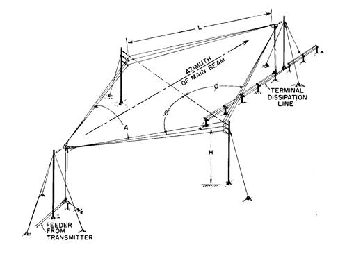
Fig. 6. 3-wire horizontal terminated rhombic antenna. Radio Antenna Engineering, p.316 (Laport, 1952).

Fig. 7 shows a graph to calculate the optimum parameters for this antenna, with the aim of maximising gain and reducing the amplitude of secondary lobes. As we can see, the leg length, the acute angle of the rhombus, the height of installation, the elevation of the main beam and the beamwidth are closely related.

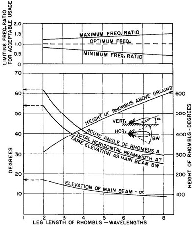
Fig. 7. Optimum parameters. Radio Antenna Engineering, p.321 (Laport, 1952).

Remark: the height of the rhombus is shown in feet.

In our example, however, we will consider the simplest case, with each side of the antenna made with only one wire.

2.2. Antenna modelling using 4NEC2.

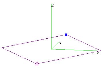
In order to design the terminated rhombic antenna in 4NEC2, we will use the same model shown in the section 1.2 (Fig. 2), adding a fifth wire segment across the open-circuit end, incorporating the terminating resistor.

We will use the following variables:

R = terminating resistance (Ω).
L = side length (metres).
A = acute angle of rhombus (degrees).
H = height of installation (metres).

The 4NEC2 antenna model is shown in Fig. 8.

Fig. 8. Terminated rhombic antenna model in 4NEC2.

Antena_Rombica_Carga.nec

2.3. Standing wave ratios.

Having the variables initialized according to the values shown in the previous sections and using a load R=600 Ω, at a frequency of 14 MHz the simulated SWR is 2.4, referenced to 300 Ω.

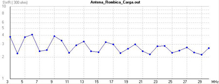
Fig. 9. SWR referenced to 300 Ω for a terminated rhombic antenna in free space, L=21.42 m and A=62°.

Fig. 9 shows the simulation results for all the HF band (3-30 MHz), using the same parameters. We can see that the SWR is markedly lower than in the previous case without the resistive load (Fig. 4). This improvement is more remarkable at the lowest frequencies.

2.4. Radiation patterns.

Fig. 10 shows the radiation pattern of the same antenna in free space, at a frequency of 14 MHz.

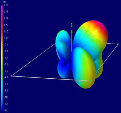
Fig. 10. Terminated rhombic antenna, free space, F=14 MHz, L=21.42 m, A=62°. 3D radiation pattern.

The main effect of terminating the antenna with a resistive load is that the radiation pattern is no longer bidirectional, but predominantly unidirectional with a lower maximum gain (3.27 dBi vs 7.44 dBi of the antenna without load). This is due to the load dissipating around half of the transmitter power. The main lobe is placed in the positive Y-axis, with an elevation of 40°.

Although we have achieved a directional pattern, due to the size and construction of the antenna it should be almost impossible to rotate, so its use is limited to fixed radio links or SIGINT stations, as was the case of the RAF "Y Stations" during the Second World War.

Fig. 11 shows the radiation patterns of the same antenna in free space, at the following frequencies: 3.8 MHz, 7 MHz, 18 MHz and 21 MHz.

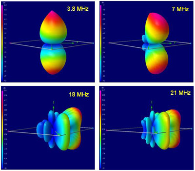
Fig. 11. Radiation patterns at several bands of interest.

At the 3.8 MHz band, the radiation pattern is completely vertical, making the antenna suitable for NVIS. However, the simulated gain is −6.2 dBi at a take-off angle of 90°.

At the 7 MHz band, the main lobe has an elevation of about 70°. The simulated gain is −3 dBi in this case.

At 18 MHz, above the design frequency (14 MHz), the simulated gain becomes positive, reaching 5.6 dBi and a main lobe with a take-off angle of 35°.

At 21 MHz, the maximum gain is 6.7 dBi and the main lobe has an elevation of 30°.

We can conclude that, although the impedance of the antenna varies slightly all along the HF band, the radiation patterns vary considerably with frequency. In practice, the design for an optimal main lobe and reduced secondary lobes can be achieved for a relatively narrow bandwidth around the design frequency.

2.5. Effects of the variation of the design parameters.

In this section we will analyse the possible effects of varying the parameters of design of the antenna: load resistance (R), length (L), acute angle of rhombus (A) and height of installation (H).

2.5.1. Load resistance.

We will analyse the changes using several different resistive loads:

F = 14 MHz.
R: 300, 600 and 900 Ω.
L = 21.42 m.
A = 62°.
H: does not have influence (free space).

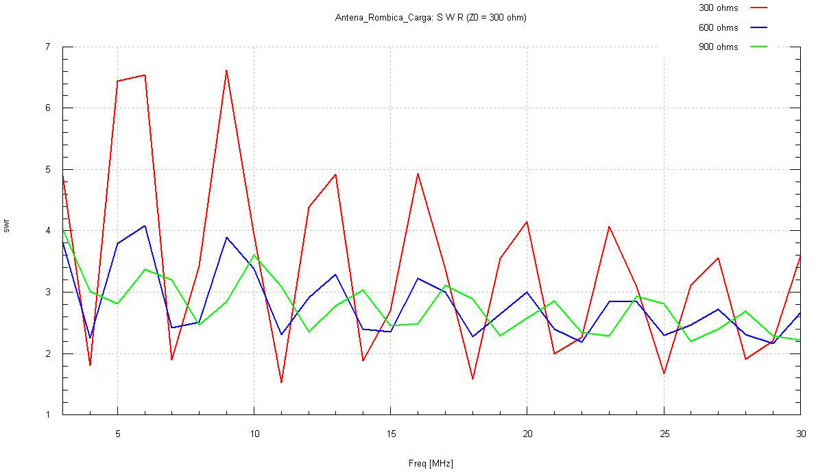
Fig. 12. SWR comparison referenced to 300 Ω in all the HF band for loads of 300, 600 and 900 Ω.

Fig. 12 shows the SWR calculated in all the HF band, using loads of 300, 600 and 900 Ω, for a characteristic impedance of 300 Ω. Click the image to view a larger version. We can see the following:

300 Ω load: the SWR (1.88) is the best at the design frequency (14 MHz), but it is quite high in several bands, especially in the lower ones, reaching values up to 6.61.

600 Ω load: the SWR gets worse at the design frequency (2.40), but is remarkably lower in all the bands, dropping as the frequency increases.

900 Ω load: at the design frequency, the SWR is slightly worse than in the previous case (3.03), but if we consider all the HF band, it is undoubtedly the better case, being the highest SWR equal to 4.02.

Fig. 13 shows a comparison of the antenna gain in all the HF band, using loads of 300, 600 and 900 Ω. The values are measured in the direction of maximum radiation, which in all the cases corresponds to the positive Y-axis and a take-off angle of 45°. Click the image to view a larger version.

Fig. 13. Comparison of the antenna gain in the HF band, using loads of 300, 600 and 900 Ω.

We can see that the value of the terminating resistance does not affect antenna gain, which on the other hand presents three different zones:

Between 3 MHz and around 9 MHz, the simulated gain is negative.
Between around 9 MHz and 26 MHz, the simulated gain is positive in the specified direction, reaching a maximum of 4.75 dBi at 17 MHz.
Between 26 MHz and 30 MHz, the simulated gain becomes negative again.

2.5.2. Leg length.

We will analyse the changes using several different leg lengths "L", that is, we will check how the size of the antenna has an influence on the SWR and the radiation pattern for a specific design frequency:

F = 14 MHz.
R = 600 Ω.
L: sweep between half wavelength (10.71 m) and three wavelengths (64.28 m).
A = 62°.
H: does not have influence (free space).

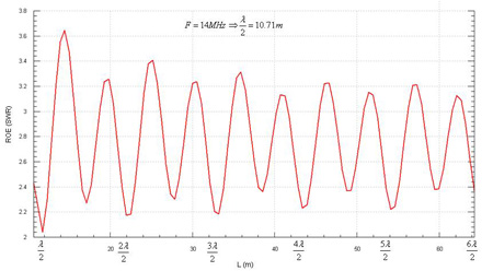
Fig. 14. SWR comparison referenced to 300 Ω at 14 MHz for different values of L.

Fig. 14 shows the SWR calculations for a characteristic impedance of 300 Ω, at a frequency of 14 MHz and for different lengths L between half wavelength and three wavelengths. See how the minimum SWR values are achieved when L is an integral number of half wavelengths at the design frequency.

Table 1 shows the maximum gain values for each L value equal to an integral number of half wavelengths (lambda) at the design frequency. The take-off angle of the main lobe of the radiation pattern is also shown.

L (0.5 × λ)	L (m)	Gain (dBi)	Take-off angle (°)
x 1	10.71	- 3	70
x 2	21.42	3.27	40
x 3	32.14	6.54	30
x 4	42.85	8.74	20
x 5	53.57	10.42	10
x 6	64.28	11.65	0

Table 1. Antenna gain and take-off angle for different values of L.

We can conclude that the antenna must be designed with a length "L" equal to an integral number of half wavelengths at the design frequency, in order to achieve the best SWR. Within those possible values, larger values of L provide higher simulated gain and lower take-off angles under the conditions studied.

2.5.3. Acute angle of rhombus.

In this section we will study the changes resulting of variations of the acute angle of the rhombus, "A", keeping constant the size of the antenna:

F = 14 MHz.
R = 600 Ω.
L = 21.42 m.
A: sweep between 30° and 90°.
H: does not have influence (free space).

Video 1 shows the results of the simulated 3D patterns. We can see that the main effect of the variations of the angle "A" is the appearance of secondary lobes approximately 90° from the direction of maximum radiation. The forward gain also changes. In a directional antenna, those secondary lobes may cause a worse signal to noise ratio in the radio communications.

Video 1. Variations of the forward gain and secondary lobes as a result of changing the acute angle of rhombus

Fig. 15 shows the plot of the forward gain (green) and the ratio between the gain of the main lobe and the gain of the secondary lobes at 90° (red). Both parameters are measured at a take-off angle of 45°. The angle "A" varies between 30° and 90°

Fig. 15. Antenna gain and comparison between lobes for different values of "A".

For small values of the angle "A", the secondary lobes are quite small, a fact quite interesting for a directional antenna. With A=30°, the ratio between the main lobe and the secondary lobes is 17 dB. However, the antenna has losses of 2 dBi in the forward direction.

On the other hand, if we select A=90° (square antenna), the forward gain will be the best (around 4.5 dBi), but the ratio between lobes is the worst (4.5 dB).

We can see that, for values around A=60°, the antenna has a forward gain of 3 dBi and the ratio between lobes is 9 dB, so we can consider this case as optimal.

Regarding SWR, the simulation shows that this parameter is scarcely related with the variations of "A".

2.5.4. Height of installation.

In this section we will analyse the variations as a result of changing the height of installation "H" of the antenna. To achieve this, we will place the antenna parallel to a perfectly conducting ground plane.

F = 14 MHz.
R = 600 Ω.
L = 21.42 m.
A = 62°.
H: sweep between 2.5 m and 53.5 m.

Video 2 shows that the main effect of this change is a variation of the elevation of the main lobe in the radiation pattern. Significant secondary lobes are created.

Video 2. Variations in the vertical radiation pattern as a result of changing the height of installation

Table 2 shows, for some selected values of "H", the relative amplitudes of the main and secondary lobes, as well as their take-off angle.

Height H (m)	Main lobe		Secondary lobes
Height H (m)	Gain (dBi)	Take-off angle (°)	Gain (dBi)	Take-off angle (°)
2.5	3.83	50	N/A	N/A
5.5	8.27	45	N/A	N/A
8.6	8.98	40	N/A	N/A
10.7 (*)	8.63	35	N/A	N/A
11.2	8.48	35	N/A	N/A
11.7	8.26	32	-19.00	75
14.2	7.57	25	-0.14	65
17.3	6.73	20	6.47	55
21.4 (*)	8.87	45	5.85	15
24.4	9.27	40	5.55	15
27.5	8.98	35	5.11 / 2.61	10 / 60
30.6	8.15	30	6.69 / 5.19	55 / 10
32.1 (*)	8.37	30	7.79 / 5.16	55 / 10
33.6	8.43	50	8.17 / 5.08	30 / 10
36.7	9.03	45	7.52 / 4.81	25 / 10
39.2	8.93	45	7.55 / 4.39 / 2.60	25 / 10 / 65
42.8 (*)	9.07	40	6.29 / 5.99 / 3.66	60 / 25 / 5
45.9	8.89	35	7.92 / 6.71 / 3.98	55 / 20 / 5
48.4	8.80	50	8.61 / 6.69 / 4.21	35 / 20 / 5
51.5	8.82	45	7.99 / 5.86 / 4.42	30 / 20 / 5
53.5 (*)	9.22	45	8.39 / 5.01 / 4.74	30 / 60 / 20

Table 2. Gain and take-off angle of the radiation lobes for selected values of H.

The marked values (*) are multiples of half wavelength at the design frequency.

We can see that the general trend is: for higher heights H, higher values of the antenna gain, although the take-off angle of the main radiation lobe will vary.

Up to a height of 11.2 m, there aren't any secondary lobes. Above this height, a secondary lobe is created, which at 14.2 m is 7 dB below the main lobe and at 24.4 m is only 3.7 dB below. From 27.5 m on, a new significant secondary lobe is created. From 33.6 m on, this secondary lobe becomes the main lobe. Finally, from 39.2 m on, there are three significant secondary lobes.

Checking all the table, if the take-off angle of the radiation pattern is a requirement of design, taking into account all the possible lobes we can cover the whole range between 5° and 60°.

3. Conclusions.

The rhombic antenna is a wideband antenna, made of two V-shaped wire sections joined at their ends and terminated in an open circuit or in a resistive load. Each side of the antenna is made of two legs of length "L" and as a whole the antenna has the shape of a rhombus, that is, the opposite angles are of the same value.

The unterminated rhombic antenna is bidirectional and has an impedance that can be matched across the HF band using an antenna tuner. The resistively terminated rhombic is predominantly unidirectional and improves SWR, but has lower gain than the unterminated version. The terminated design operates as a travelling-wave antenna, whereas the unterminated version exhibits reflections and standing waves.

Although the antenna has the important advantage of presenting an impedance with slight variations in all the HF band, the radiation patterns vary considerably with frequency, showing changes in the gain, the take-off angle of the main lobe and the number of secondary lobes, which in some cases may present significant amplitudes.

Several simulations have been performed, taking into account the following parameters of design:

F: design frequency (MHz).
L: side length (m).
A: acute angle of rhombus (degrees).
R: terminating resistance (Ω).
H: height of installation (m).

Table 3 shows the effects of all those parameters in the design of the antenna.

	SWR	Gain	Take-off angle	Secondary lobes
R	Yes	No	No	Rear lobes only
L	Yes	Yes	Yes	Yes
A	No	Yes	Yes	Yes
H	Negligible	Yes	Yes	Yes

Table 3. Effects of the parameters of design for rhombic antennas.

The rhombic antennas can be considered as wideband antennas from the impedance point of view, but the radiation patterns vary considerably with frequency. Due to those facts, this kind of antennas must be optimized to be used at particular frequencies.